<?xml version="1.0" encoding="utf-8"?><feed xmlns="http://www.w3.org/2005/Atom" ><generator uri="https://jekyllrb.com/" version="3.10.0">Jekyll</generator><link href="https://vzahorui.github.io/feed.xml" rel="self" type="application/atom+xml" /><link href="https://vzahorui.github.io/" rel="alternate" type="text/html" /><updated>2026-06-07T16:11:32+00:00</updated><id>https://vzahorui.github.io/feed.xml</id><title type="html">Unlocking the power of data</title><subtitle>Knowledge base related to data science. In depth description of statistical concepts and machine learning models.</subtitle><author><name>Vladyslav Zahorui</name></author><entry><title type="html">Generalized Linear Models</title><link href="https://vzahorui.github.io/regression/generalized-linear-regression/" rel="alternate" type="text/html" title="Generalized Linear Models" /><published>2026-01-25T00:00:00+00:00</published><updated>2026-01-25T00:00:00+00:00</updated><id>https://vzahorui.github.io/regression/generalized-linear-regression</id><content type="html" xml:base="https://vzahorui.github.io/regression/generalized-linear-regression/"><![CDATA[<p>Generalized Linear Models (GLMs) provide a powerful and flexible framework for modeling a response variable ($Y$) that is non-normally distributed or related to the predictors ($X$) in a nonlinear way. GLMs generalize <a href="/regression/linear-regression/">Ordinary Least Squares</a> (OLS) regression by allowing for response variables that have error distribution models other than a <a href="/probability%20&amp;%20statistics/normal-distribution/">normal distribution</a>.</p>

<p>In standard linear regression, we assume the response variable $Y$ can range from $−\infty$ to $+\infty$. However, real-world data is often restricted, for example:</p>

<ul>
  <li>Probabilities (<a href="/probability%20&amp;%20statistics/statistical-distributions/#binomial_distribution">Binary</a> data) must be between 0 and 1.</li>
  <li>Counts (<a href="/probability%20&amp;%20statistics/statistical-distributions/#poisson_distribution">Poisson</a> data) must be positive integers.</li>
</ul>

<p>If we tried to predict these directly with a linear equation $X \beta$ (which is unbounded), we might predict a probability of -0.5 or a count of -10, which is physically impossible.</p>

<h2 id="components-of-glm">Components of GLM</h2>

<p>A GLM consists of three key components:</p>

<ol>
  <li>
    <p>Random Component: The <a href="/probability%20&amp;%20statistics/statistical-distributions/">probability distribution</a> of the response variable, $Y$, must belong to the Exponential Family of Distributions.</p>
  </li>
  <li>
    <p>Systematic Component (Linear Predictor): A linear combination of the predictor variables, $\eta=x^T \beta$.</p>
  </li>
  <li>
    <p>Link Function: A function, $g(⋅)$, that maps the bounded expected value of the response, $\mu=E[Y]$, to the linear predictor: $g(\mu)=\eta$.</p>
  </li>
</ol>

<p>It is important to realize that each observation is drawn from a separate distribution which is determined by the predictor variables $X$. Even though the aim of the regression is to estimate the common parameters $\beta$, each observation has its individual $X$ variables which in turn define a separate distribution (sharing the same family, but with unique mean and variance parameters).</p>

<p>During model fitting, we view the observed data $Y$ as a random realization drawn from these distributions, while the model attempts to estimate the underlying vector of means $\mu$ that generated them.</p>

<h2 id="the-exponential-family-of-distributions">The Exponential Family of Distributions</h2>

<h3 id="the-foundation">The Foundation</h3>

<p>The Random Component of a GLM relies entirely on the Exponential Family of Distributions. This is a class of probability distributions (including Normal, Poisson, Binomial, Gamma, etc.) whose density/mass function can be written in the standardized, canonical form:</p>

\[f(y; \theta, \phi) = \exp \left(\frac{y \theta - b(\theta)}{a(\phi)} + c(y, \phi) \right)\]

<ul>
  <li>$\theta$ (Canonical Parameter) relates to the mean $\mu$ of the distribution and represents the “location” of the distribution.</li>
  <li>$y \theta$ (Interaction) “rewards” the likelihood function. If both the observation $y$ and the parameter $\theta$ are large and positive, the exponent increases, maximizing the probability.</li>
  <li>$b(\theta)$ (Cumulant) is a convex function which balances $y \theta$ by not letting it increase to infinity during the optimization $\theta$.</li>
  <li>$a(\phi)$ (Dispersion) is a function of a dispersion parameter $\phi$ (often the variance, $\sigma^2$). It scales the distribution.</li>
  <li>$c(y, \phi)$ is a normalization term for the data structure itself (e.g., factorials or constants). It encodes properties which do not depend on $\theta$, and thus on the mean.</li>
</ul>

<h3 id="the-utility-of-the-exponential-family">The Utility of the Exponential Family</h3>

<p>The canonical form of Exponential Family yields a unified set of mathematical properties essential for efficient model fitting.</p>

<h4 id="mean-variance-relationship">Mean-Variance Relationship</h4>

<p>The mean ($\mu$) and the variance ($V$) of the distribution are directly defined by the cumulant function $b(\theta)$ and the dispersion parameter $\phi$.</p>

<ul>
  <li>Mean: $E[Y]=b’(\theta)$</li>
  <li>Variance: $Var(Y)=b’’(\theta) \cdot a(\phi)$</li>
</ul>

<h5 id="deriving-the-mean">Deriving the Mean</h5>

<p>If $f(y; \theta)$ is a probability density, its <a href="/calculus/integrals/">integral</a> over all possible values of $y$ is 1.</p>

\[\int \exp \left(\frac{y \theta - b(\theta)}{a(\phi)} + c(y, \phi) \right) dy = 1\]

<p>We can put both sides under the <a href="/calculus/derivatives/">derivative</a> with respect to $\theta$ and land with this equation:</p>

\[\frac{d}{d\theta} \int \exp \left(\frac{y \theta - b(\theta)}{a(\phi)} + c(y, \phi) \right) dy = 0\]

<p>By putting the derivative under the integral and by applying the chain rule we get this:</p>

\[\int f(y; \theta) \cdot \left(\frac{y}{a(\phi)} - \frac{'b(\theta)}{a(\phi)}\right) dy = 0\]

<p>And then by distributing and rearranging:</p>

\[\int \frac{y}{a(\phi)} \cdot f(y; \theta) dy = \int \frac{'b(\theta)}{a(\phi)} \cdot f(y; \theta) dy\]

\[\int y \cdot f(y; \theta) dy = \int b'(\theta) \cdot f(y; \theta) dy\]

<p>The expression on the left is the expected value of $Y$. In the second term, $b’(\theta)$ is a constant (it doesn’t depend on $y$), so it pulls out. What’s left is simply the integral over the density function which equals 1.</p>

<p>And therefore,</p>

\[E[Y]=b'(\theta)\]

<h5 id="deriving-the-variance">Deriving the Variance</h5>

<p>We start from our previous result: $\int f(y; \theta) \cdot \left(\frac{y}{a(\phi)} - \frac{‘b(\theta)}{a(\phi)}\right) dy = 0$. This expression is differentiated from both sides with respect to $\theta$ using the product rule ($uv’ + u’v$).</p>

\[\int -\frac{b''(\theta)}{a(\phi)} f(y; \theta) dy + \int \left(\frac{y}{a(\phi)} - \frac{'b(\theta)}{a(\phi)}\right)^2 f(y; \theta) dy = 0\]

<p>Then again, considering that the integral over the density function which equals 1 and by rearranging we get this:</p>

\[\frac{1}{a(\phi)^2} \int \left(y - 'b(\theta)\right)^2 f(y; \theta) dy = \frac{b''(\theta)}{a(\phi)}\]

\[\int \left(y - \mu \right)^2 f(y; \theta) dy = b''(\theta) \cdot a(\phi)\]

<p>The expression on the left is the variance of $Y$. Therefore,</p>

\[Var[Y]=b''(\theta) \cdot a(\phi)\]

<h4 id="sufficient-statistics-data-compression">Sufficient Statistics (Data Compression)</h4>

<p>This is a critical property for Big Data. Because the data $y$ enters the probability formula only through the linear product $y \theta$, the likelihood can be factored.</p>

<p>Below you can find details on the maximum likelihood estimation but here it suffices to say that if the Canonical Link is used (where $\theta=X\beta$), the term becomes $y(X\beta)$. This means the sum $\sum y_{i} ​x_{ij}$​ is a sufficient statistic for $\beta$.</p>

<p>This means that the algorithm does not need to store millions of raw rows in memory; it can compress the entire dataset into a simple vector of sums to perform the optimization.</p>

<h4 id="canonical-link-function">Canonical Link Function</h4>

<p>The canonical link function $g_{\text{canonical}}​(\mu)$ is the specific link that maps the mean directly to the canonical parameter:</p>

\[g_{\text{canonical}}​(\mu)=\theta\]

<p>In this case $\theta$ is linearly modeled as $x^{T} \beta$. So essentially $\theta = \eta$.</p>

<p>Since $\mu = b’(\theta)$, the canonical link function $g_{\text{canonical}}​(\mu)$ is the inverse function of  $b’(\theta)$.</p>

<p>Here is an overview of the common canonical link functions:</p>

<table>
  <thead>
    <tr>
      <th style="text-align: center">Distribution</th>
      <th style="text-align: center">Type of Data</th>
      <th style="text-align: center">$Var(Y)$</th>
      <th style="text-align: center">Canonical link $g_c(\mu) = \theta$</th>
      <th style="text-align: center">Application</th>
    </tr>
  </thead>
  <tbody>
    <tr>
      <td style="text-align: center">Normal</td>
      <td style="text-align: center">Continuous, Unbounded</td>
      <td style="text-align: center">$\phi$ (constant variance)</td>
      <td style="text-align: center">Identity: $\mu$</td>
      <td style="text-align: center">Classic Linear Regression (OLS)</td>
    </tr>
    <tr>
      <td style="text-align: center"><a href="/probability%20&amp;%20statistics/statistical-distributions/#poisson_distribution">Poisson</a></td>
      <td style="text-align: center">Count data</td>
      <td style="text-align: center">$\mu$ (variance equals mean)</td>
      <td style="text-align: center">$\log(\mu)$</td>
      <td style="text-align: center">Modeling counts of events: website clicks, call center arrivals, number of accidents, disease incidence rates.</td>
    </tr>
    <tr>
      <td style="text-align: center"><a href="/probability%20&amp;%20statistics/statistical-distributions/#binomial_distribution">Binomial</a></td>
      <td style="text-align: center">Binary/Proportion Data (Out of $N$ Trials)</td>
      <td style="text-align: center">$\frac{\mu(1-\mu)}{N}$</td>
      <td style="text-align: center">Logit: $\log(\frac{\mu}{1-\mu})$</td>
      <td style="text-align: center">Modeling probabilities/proportions: survival rate, proportion of successes, customer churn probability, Yes/No responses (Logistic Regression).</td>
    </tr>
    <tr>
      <td style="text-align: center">Gamma</td>
      <td style="text-align: center">Continuous, Positive, Right-Skewed</td>
      <td style="text-align: center">$\mu^2 \phi$</td>
      <td style="text-align: center">$\frac{1}{\mu}$</td>
      <td style="text-align: center">Modeling non-negative, non-count data: insurance claim amounts, rainfall totals, income (when modeling the mean).</td>
    </tr>
    <tr>
      <td style="text-align: center">Inverse Gaussian</td>
      <td style="text-align: center">Continuous, Positive, Highly Skewed</td>
      <td style="text-align: center">$\mu^3 \phi$</td>
      <td style="text-align: center">$\frac{1}{\mu^2}$</td>
      <td style="text-align: center">Modeling first passage times in stochastic processes: time to failure/default, survival analysis, financial duration modeling, highly skewed physical data.</td>
    </tr>
  </tbody>
</table>

<h5 id="other-important-non-canonical-models">Other Important (Non-Canonical) Models</h5>

<p>Sometimes, the distribution’s theoretical variance structure is deemed inappropriate for the data, but the mean structure is fine. This leads to commonly used extensions:</p>

<table>
  <thead>
    <tr>
      <th style="text-align: center">Distribution</th>
      <th style="text-align: center">Canonical Link Function</th>
      <th style="text-align: center">$Var(Y)$</th>
      <th style="text-align: center">Why Use It?</th>
    </tr>
  </thead>
  <tbody>
    <tr>
      <td style="text-align: center"><a href="/probability%20&amp;%20statistics/statistical-distributions/#negative_binomial_distribution">Negative Binomial</a></td>
      <td style="text-align: center">Log</td>
      <td style="text-align: center">$\mu + \alpha \mu^2$ ($\alpha &gt; 0$)</td>
      <td style="text-align: center">Used for Overdispersed Count Data where the variance is significantly greater than the mean.</td>
    </tr>
    <tr>
      <td style="text-align: center">Quasi-Binomial</td>
      <td style="text-align: center">Logit</td>
      <td style="text-align: center">$\phi \frac{\mu (1-\mu)}{N}$</td>
      <td style="text-align: center">Used for Over/Underdispersed Proportion Data (e.g., in ecological or developmental studies where variance is too high or too low).</td>
    </tr>
  </tbody>
</table>

<h4 id="maximum-likelihood-estimation-mle-simplification">Maximum Likelihood Estimation (MLE) Simplification</h4>

<p>Using the canonical form results in a concave log-likelihood function, which guarantees a unique global maximum. This makes the MLE process simpler and more robust. More to it the section below.</p>

<h2 id="maximul-likelihood-estimation">Maximul Likelihood Estimation</h2>

<p>In GLMs, the model parameters $\beta$ (the coefficients) are estimated using <a href="/optimization/maximum-likelihood/">Maximum Likelihood Estimation</a> (MLE). The goal of MLE is to find the values of $\beta$ that make the observed data most probable.</p>

<h3 id="the-likelihood-and-log-likelihood-functions">The Likelihood and Log-Likelihood Functions</h3>

<p>For a set of $n$ independent observations $Y=(y_1​,y_2​,…,y_n​)$, the Likelihood Function, $\mathcal{L}(\beta∣Y)$, is the product of the individual density/mass functions at each observation, $f(y_i​)$, where each $f(y_i​)$ is parameterized by a unique $\theta_i$​ that depends on $\beta$ via the link function:</p>

\[\mathcal{L}(\beta∣Y)=\prod_{i=1}^n ​f(y_i​;\theta_i​)\]

<p>For computational simplicity (turning a product into a sum) and numerical stability, we maximize the Log-Likelihood Function:</p>

\[l(\beta∣Y)= \sum_{i=1}^n \log (​f(y_i​;\theta_i​))\]

<p>Expanding the density function with the canonical form of Exponential Family:</p>

\[l(\beta∣Y)= \sum_{i=1}^n \left(\frac{y_i \theta_i - b(\theta_i)}{a(\phi_i)} + c(y_i, \phi_i) \right)\]

<ul>
  <li>The first term, $\sum_{i=1}^n \frac{y_i \theta_i - b(\theta_i)}{a(\phi_i)}$​, is the kernel of the log-likelihood and contains all the terms dependent on the parameters $\beta$ (since $\theta$​ is a function of $\beta$).</li>
  <li>The second term, $\sum_{i=1}^n c(y_, \phi_i)$, does not depend on the regression coefficients $\beta$, so it can be ignored when solving for the MLEs.</li>
</ul>

<p>Therefore, the likelihood is proportionate to this construct:</p>

\[l(β) \propto \sum_{i=1}^n ​(y_i \theta_i - b(\theta_i))\]

<h3 id="the-maximization-process-finding-the-score">The Maximization Process (Finding the Score)</h3>

<p>To find the values of $\beta$ that maximize the log-likelihood, we take the partial <a href="/calculus/derivatives/">derivative</a> of $l(\beta)$ with respect to each $\beta_j$​ and set the resulting expression (the Score Function) equal to zero:</p>

\[U(\beta_j) = \frac{\partial l}{\partial \beta_j} = 0\]

<p>Using the chain rule, the score equation becomes:</p>

\[\frac{\partial l}{\partial \beta_j} = \frac{\partial l}{\partial \theta} \cdot \frac{\partial \theta}{\partial \mu} \cdot \frac{\partial \mu}{\partial \eta} \cdot \frac{\partial \eta}{\partial \beta_j}\]

<p>From deriving the mean and the variance of $Y$ in the section above we know that $\mu = b’(\theta)$, therefore $\frac{\partial \mu}{\partial \theta} = b’’(\theta)$. We also know that $Var(Y) = b’’(\theta) \cdot a(\phi)$, thus $\frac{\partial \mu}{\partial \theta} = \frac{Var(Y)}{a(\phi)}$. Inverting this gives us the term we need:
$\frac{\partial \theta}{\partial \mu} = \frac{a(\phi)}{Var(Y)}$.</p>

<p>By applying it to the equation above we arrive at the general score equation:</p>

\[\sum_{i=1}^n \left[\frac{y_i - \mu_i}{Var(Y_i)} \cdot \frac{\partial \mu_i}{\partial \eta_i} \cdot x_{ij} \right] = 0\]

<p>Intuitively, the variance appearing in the denominator acts as a weighting mechanism. The term $(y−\mu)$ is the error (residual), while the term $1/Var(Y)$ down-weights observations that are naturally noisy. In this way the model “tries harder” to fit observations with low variance and “forgets” about observations with high variance.</p>

<h4 id="simplification-with-the-canonical-link">Simplification with the Canonical Link</h4>

<p>We can expand a part of the chain rule described above as this:</p>

\[\frac{\partial \mu_i}{\partial \eta_i} = \frac{\partial \mu_i}{\partial \theta_i} \cdot \frac{\partial \theta_i}{\partial \eta_i}\]

<p>Then if we use the Canonical Link ($g_c​(\mu)=\theta$), we have $\mu=b’(\theta)$ and $\theta=\eta$. Therefore the expression above simplifies as follows:</p>

\[\frac{\partial \mu_i}{\partial \eta_i} = b''(\theta) \cdot 1 = \frac{Var(Y)}{a(\phi)}\]

<p>When putting this into the original score equation the terms $Var(Y)$ cancels out. Considering that $a(\phi)$ is constant we have this simpliefied form:</p>

\[\sum_{i=1}^n (y_i - \mu_i) x_{ij} = 0\]

<p>This removal of the complex non-linear variance term from the denominator is why canonical link models are so computationally robust and guaranteed to converge, and why we can utilize the sufficient statistic by aggregating the data.</p>

<h3 id="solving-the-equation">Solving the Equation</h3>

<p>The score equation has no closed-form solution (except for a few special cases like <a href="/regression/linear-least-squares/">OLS</a> and Poisson regression with a canonical link). Since the Score Equation is non-linear, we use an iterative algorithm called Fisher Scoring (or Newton-Raphson), which can be expressed as Iteratively Reweighted Least Squares (IRLS).</p>

<p>Recall the multivariate <a href="/optimization/newton-method/">Newton’s update rule</a> for a parameter vector $\beta$:</p>

\[\beta_t = \beta_{t-1} - \left[Hf(\beta_{t-1}) \right]^{-1} \Delta f(\beta_{t-1})\]

<p>In the context of GLMs, we are maximizing the <a href="/optimization/maximum-likelihood/">log-likelihood</a> $l(\beta)$. Therefore the <a href="/calculus/derivatives/">gradient</a> $\Delta f$ is the Score Function $U(\beta)$, and the the hessian $Hf$ is the matrix of second derivatives. In practice, we often use the Expected Hessian (the negative <a href="/probability%20&amp;%20statistics/fisher-information/">Fisher Information Matrix</a>), a variation known as Fisher Scoring.</p>

<p>Substituting these into the Newton formula, the update becomes:</p>

\[\beta_t = \beta_{t-1} + \left[I(\beta_{t-1}) \right]^{-1} U(\beta_{t-1})\]

<h4 id="elaboration-on-fisher-information">Elaboration on Fisher Information</h4>

<p>For a GLM, the Information Matrix is derived as the variance of the Score Function (the gradient of the log-likelihood). It takes the form of a “weighted sandwich” of your data:</p>

\[I(\beta) = X^T WX =\sum_{i=1}^N x_i W_i x_{i}^{T}\]

<p>where</p>

<ul>
  <li>$N$ is the total number of observations.</li>
  <li>$x_i$ is the vector of predictors for observation $i$ (the $i$-th row of the design matrix $X$).</li>
  <li>$W_i$ is the Working Weight for observation i, defined as:</li>
</ul>

\[W_i = \frac{1}{Var(Y_i)} \left(\frac{\partial \mu_i}{\partial \eta_i}\right)^2\]

<p>The weight $W_i$ is the mathematical result of the Fisher Information of a single observation. It accounts for two critical factors:</p>

<ol>
  <li>
    <p>Precision $\frac{1}{Var(Y_i)}$: This term accounts for the mean-variance relationship of the chosen distribution. Observations with higher predicted variance are considered “noisier” and are down-weighted.</p>
  </li>
  <li>
    <p>Sensitivity $\left(\frac{\partial \mu_i}{\partial \eta_i}\right)^2$: This derivative reflects the link function’s curvature. Observations where a small change in the linear predictor $\eta$ leads to a large change in the mean $\mu$ are more informative and receive higher weight.</p>
  </li>
</ol>

<h4 id="linearization-for-the-newton-update">Linearization for the Newton Update</h4>

<p>Due to the non-linear link function, the variable $y$ which we want to predict lives in another dimension as the linear predictor $\eta = X \beta$. Therefore we set $z$ as a First-order [Taylor expansion(/calculus/taylor-series/)] of the link function $g(y)$ around the current mean $\mu$:</p>

\[z_i \approx g(\mu_i) + (y_i - \mu_i) g'(\mu_i)\]

\[z_i \approx \eta_i + (y_i - \mu_i) \frac{\partial \eta_i}{\partial \mu_i}\]

<p>This produces the Working Dependent Variable. Intuitively it’s a current linear prediction $\eta$, adjusted by the current error $(y−\mu)$, which has been “stretched” or “shrunk” by the slope of the link function. By making approximation $y \approx z$ we transition from the outcome space of $y$ to a linear dimension, and the error $(y−\mu)$ is translated into the same space.</p>

<p>Now let’s look again at the score equation. We can force $W$ into it by multiplying and dividing by $\frac{\partial \mu_i}{\partial \eta_i}$:</p>

\[U_i = \left[\frac{1}{Var(Y_i)}  \left(\frac{\partial \mu_i}{\partial \eta_i}\right)^2 \right] \cdot \left[(y_i - \mu_i) \frac{\partial \eta_i}{\partial \mu_i} \right] \cdot x_i\]

\[U_i = X^T W e\]

<p>where $e$ is the vector of scaled errors. From the expression of the Working Dependent Variable $e$ is equivalent to $(z - \eta)$.</p>

<h4 id="putting-it-all-together">Putting it all together</h4>

<p>By plugging the information matrix, and the linearized score function into the newton update we get this equation:</p>

\[\beta_t = \beta_{t-1} + \left(X^T W X \right)^{-1} X^T W (z - \eta)\]

<p>Then when we redistribute $\left(X^T W X \right)^{-1} X^T W$ across $(z - \eta)$, the part involving $\eta$ (which is $X \beta_{t-1}$) becomes negative $\beta_{t-1}$. Which simplifies to this:</p>

\[\beta_t = \left(X^T W X \right)^{-1} X^T W z\]

<h4 id="the-algorithm-steps">The Algorithm Steps</h4>

<ol>
  <li>
    <p>Initialize: Start with an initial guess for $\beta$.</p>
  </li>
  <li>
    <p>Calculate $\mu$ and $W$: Use the current $\beta$ to calculate the predicted means and the weights based on the chosen distribution.</p>
  </li>
  <li>
    <p>Construct $z$: Form the working dependent variable using the residuals and the link function derivative.</p>
  </li>
  <li>
    <p>Solve WLS: Calculate the new $\beta$ using the WLS formula.</p>
  </li>
  <li>
    <p>Repeat: Iterate until the change in $\beta$ is smaller than a pre-defined threshold (convergence).</p>
  </li>
</ol>

<h2 id="standard-error-of-coefficients">Standard Error of Coefficients</h2>

<p>In <a href="/probability%20&amp;%20statistics/probability-statistics/">statistics</a>, the variance of an estimator (like a regression coefficient) is inversely related to the amount of information the data contains about that parameter. This relationship is tied to the shape of the likelihood function: the more sharply peaked the likelihood function is at its maximum, the more “certain” we are of the estimate. A sharper peak corresponds to a smaller variance and, consequently, a smaller standard error.</p>

<p>The matrix that mathematically quantifies this information—and specifically the curvature of the log-likelihood—is called the <a href="/probability%20&amp;%20statistics/fisher-information/">Fisher Information Matrix</a>, $I(\beta)$. The estimated variance-covariance matrix for the coefficients, $V(\hat \beta)$, is obtained by inverting the Information Matrix at the final Maximum Likelihood estimates:</p>

\[V(\hat \beta) = I(\hat \beta)^{-1}\]

<p>The diagonal elements of $V(\hat \beta)$, provide the variances of individual coefficients, and their square roots are the Standard Errors you see in model output.</p>

<h2 id="generalized-estimating-equations-gee">Generalized Estimating Equations (GEE)</h2>

<p>Standard Generalized Linear Models (GLMs) have a crucial assumption:</p>

<ul>
  <li>Independence: All observations ($Y_i$​) are independent of each other, conditional on the covariates.</li>
</ul>

<p>This assumption is violated when data is <a href="/clustering/clustering-overview/">clustered</a> (grouped) or longitudinal (repeated measures over time on the same subject). An example of clustered data is student test scores clustered within a classroom. Students in the same classroom are likely more similar due to the same teacher, curriculum, and environment.</p>

<p>In these cases, fitting a standard GLM (like logistic or Poisson regression) is problematic because the     standard errors of coefficients (and thus p-values and <a href="/probability%20&amp;%20statistics/sampling-distribution/#confidence_interval">confidence intervals</a>) will be incorrectly small, leading to an inflated sense of precision and potentially false conclusions of statistical significance.</p>

<p>Generalized Estimating Equations (GEE) provide a robust, non-likelihood-based approach to analyzing clustered or longitudinal data where observations within groups are correlated. It is an extension of the GLM framework, but with a critical focus on getting the standard errors correct.</p>

<h3 id="how-gee-works">How GEE works</h3>

<p>Suppose you have 10 different classrooms, each with 30 students. You want to determine if spending more time on homework (your covariate) leads to better test scores.</p>

<ol>
  <li>
    <p><strong>Initial Estimate</strong>: GEE begins exactly like a standard GLM by calculating the initial coefficients $\beta^{(0)}$. For example, it might estimate that for every extra hour of homework, scores increase by 5 points. This estimate is usually unbiased even if the internal correlation is initially ignored.</p>
  </li>
  <li>
    <p><strong>Define Correlation Structure</strong>: You must define a “working correlation structure” ($R$) that describes how students within the same classroom are related.</p>
  </li>
</ol>

<p>A common choice is Exchangeable (Compound Symmetry), which assumes every pair of students in a class shares the same correlation level, $\alpha$. At this stage, you only define the shape of the matrix; the actual numerical value of $\alpha$ is estimated later from the data.</p>

<p>The following steps are then repeated until the coefficients converge:</p>

<p>Note, each cluster is processed separately.</p>

<ol>
  <li><strong>Calculate Means and Variances ($A_i$​)</strong>: Using the current coefficient estimate $\beta^{(t−1)}$, we calculate the cluster mean vector $\mu_i$​ and the variance matrix $A_i$​.</li>
</ol>

\[\mu_i^{(t-1)} = g^{-1}(X_i \beta^{(t−1)})\]

<p>$A_i$ is a diagonal matrix where each entry is the variance of a single observation based on the distribution’s mean-variance relationship (e.g., for Poisson, the variance is simply $μ_{ij}$​).</p>

\[A_i​=\text{diag}(V(\mu_{i1}​),V(\mu_{i2}​),…,V(\mu_{in}​))\]

<ol>
  <li><strong>Calculate and Standardize Residuals</strong>: We determine the raw residuals $S_i$​ and then “standardize” them by dividing the error by the predicted standard deviation (from matrix $A$):</li>
</ol>

\[S_i^{(t-1)}= Y_i - \mu_i^{(t-1)}\]

\[r_{ij} = \frac{y_{ij}-\mu_{ij}}{\sqrt{V(\mu_{ij})}}\]

<ol>
  <li><strong>Update Global Parameters ($\alpha$ and $\phi$)</strong>: These are global parameters shared across all clusters. While each classroom has its own data, the “rules of the game”—the noise level ($\phi$) and the correlation strength ($\alpha$)—are estimated as single values for the entire dataset.</li>
</ol>

<p>$\phi$ accounts for overdispersion (when data is noisier than theoretically expected). It is calculated from the average of the squared Pearson residuals:</p>

\[\phi = \frac{1}{N - p} \sum_{i=1}^{K} \sum_{j=1}^{n_i} r_{ij}^2\]

<p>here</p>

<ul>
  <li>$N$ is the total number of observations.</li>
  <li>$p$ is number of regression coefficients ($\beta$).</li>
</ul>

<p>If $\phi$ is 1, the data matches the theoretical variance perfectly. If it is equal 2, the data is twice as noisy as a standard Poisson/Binomial distribution would expect. GEE uses this to “inflate” the standard errors so you don’t overstate your confidence.</p>

<p>$\alpha$ is estimated by looking at the “co-movement” of residuals within the same cluster. For the Exchangeable structure (where every pair has the same correlation), we sum the products of residuals for all possible pairs within each cluster:</p>

\[\alpha = \frac{1}{\text{Total pairs} \cdot \phi} \sum_{i=1}^K \sum_{j&gt;k} r_{ij} r_{ik}\]

<p>If student $j$ and student $k$ consistently both have “higher than expected” scores (positive $r$ $\times$ positive $r$) or “lower than expected” scores (negative $r$ $\times$ negative $r$), the product is positive, and $$alpha$ goes up. If their residuals are totally unrelated, the positive and negative products cancel out, and $\alpha$ stays near zero.</p>

<ol>
  <li><strong>Construct Cluster Covariance ($V_i$​)</strong>: We combine the theoretical variance ($A_i$​), the correlation structure ($R_i$​), and the dispersion ($\phi$) into a single covariance matrix for the cluster:</li>
</ol>

\[V_i^{t} = \phi A_i^{1/2} R_i(\hat \alpha^{(t)}) A_i^{1/2}\]

<ul>
  <li>$A_i^{1/2}$ is diagonal matrix where the j-th diagonal entry is the square root of the GLM variance</li>
</ul>

<p>$V_i^{t}$​ represents the total estimated variance of the response vector $Y_i$​, accounting for both the distribution type and the clustering effect.</p>

<ol>
  <li><strong>Update Coefficients ($\beta$)</strong>: Finally, we solve the Generalized Estimating Equation to find the new estimate $β^{(t)}$:</li>
</ol>

\[U(\beta^{(t)})=  \sum_{i=1}^K ​D_i^T​ (V_i^{t}​)^{−1} (Y_i​−\mu_i^{(t)}​)=0\]

<p>Here $D_i$ is the derivative matrix $\frac{\partial \mu_i}{\partial \beta}$. It acts like the design matrix X but is “adjusted” for the link function. (In the standard GLM section, this derivative was included within the weight matrix $W$, allowing for the use of the “clean” $X$ matrix instead).</p>

<p>This non-linear equation is solved iteratively (via Newton-Raphson or Fisher Scoring), approximating the solution as:</p>

\[\beta^{(t)}=\beta^{(t-1)}+ \left[\sum_{i=1}^{K} ​D_i^T ​(V_i^{t}​)^{−1} D_i \right]^{-1} \sum_{i=1}^{K} ​D_i^T ​(V_i^{t}​)^{−1} S_i^{(t−1)​}\]

<h3 id="robust-estimation-of-parameters-covariance">Robust Estimation of Parameters Covariance</h3>

<p>Once the $\hat \beta$​ has converged, the final step is to calculate the robust standard errors, which are necessary for hypothesis testing and confidence intervals.</p>

<p>The Robust (Sandwich) Covariance Matrix for $\hat \beta$​ is calculated as:</p>

\[V_{\text{robust}}(\hat \beta) = B^{-1} C B^{-1}\]

<p>The standard errors for the coefficients are the square roots of the diagonal elements of this matrix.</p>

<h4 id="b-the-bread-or-model-based-part">$B$ (The Bread, or Model-Based Part)</h4>

<p>This is the term calculated from the final iteration of the fitting process. It represents the Model-Based (or Naive) covariance estimate.</p>

\[B = \sum_{i=1}^{K} ​D_i^T ​(V_i^{t}​)^{−1} D_i\]

<p>This is exactly the same “Information Matrix” we discussed for standard GLMs ($X^{T}WX$). In GEE, it represents what the variance of your coefficients should be if your “guess” about the correlation ($V_i$​) was 100% correct. It’s called the “Bread” because it surrounds the center. In a perfect world where your model is perfect, the variance would just be $B^{−1}$.</p>

<h4 id="c-the-meat-or-empirical-part">$C$ (The Meat, or Empirical Part)</h4>

<p>This matrix captures the observed variability between the clusters, making no assumptions about the internal correlation structure. It is the sum of the outer products of the weighted residuals from each cluster.</p>

\[C = \sum_{i=1}^{K} ​D_i^T ​V_{i}​^{-1} S_i S_i^T V_i^{-1} D_i\]

<p>$S_i S_i^T$: This is the “outer product” of the residuals. While $V_i$​ is what your model thinks the covariance is, $S_i S_i^T$ is the actual, raw covariance observed in the data for that cluster.</p>

<p>For example, if students in Classroom 5 are much more similar to each other than your model predicted, $S_i S_i^T$ will be much larger than $V_i$​.</p>

<p>If S_i S_i^T$ is equal to $V_i$ then the “meat” simplifies and becomes equal to $B$. Consequently, the robust estimator is simply $B^{-1}$, same as the standard GLM variance.</p>

<p>The beauty of the Sandwich Estimator is its consistency. Even if the “working” correlation structure $V_i$​ is specified incorrectly, the Meat ($C$) uses the actual observed residuals to correct the Model-Based Bread ($B$). As long as your sample size of clusters ($K$) is sufficiently large, the resulting standard errors will be asymptotically correct.</p>]]></content><author><name>Vladyslav Zahorui</name></author><category term="Regression" /><category term="statistics" /><category term="linear-regression" /><category term="GLM" /><category term="OLS" /><category term="probability-density-function" /><category term="probability-mass-function" /><category term="normal-distribution" /><category term="maximum-likelihood-estimation" /><category term="MLE" /><category term="iteratively-reweighted-least-squares" /><category term="IRLS" /><category term="generalized-estimating-equations" /><category term="GEE" /><category term="information-matrix" /><category term="standard-error" /><category term="sandwitch-estimator" /><category term="Fisher-information" /><summary type="html"><![CDATA[Generalized Linear Models (GLMs) provide a powerful and flexible framework for modeling a response variable ($Y$) that is non-normally distributed or related to the predictors ($X$) in a nonlinear way. GLMs generalize Ordinary Least Squares (OLS) regression by allowing for response variables that have error distribution models other than a normal distribution.]]></summary></entry><entry><title type="html">Fisher Information</title><link href="https://vzahorui.github.io/probability%20&%20statistics/fisher-information/" rel="alternate" type="text/html" title="Fisher Information" /><published>2025-12-26T00:00:00+00:00</published><updated>2025-12-26T00:00:00+00:00</updated><id>https://vzahorui.github.io/probability%20&amp;%20statistics/fisher-information</id><content type="html" xml:base="https://vzahorui.github.io/probability%20&amp;%20statistics/fisher-information/"><![CDATA[<p>Fisher Information, denoted $I(\theta)$, is a foundational concept in mathematical <a href="/probability%20&amp;%20statistics/probability-statistics/">statistics</a>. It quantifies the amount of information that an observable random variable $X$ carries about an unknown parameter $\theta$ of its <a href="/probability%20&amp;%20statistics/statistical-distributions/">probability distribution</a>.</p>

<p>Essentially, Fisher Information measures how sensitive the <a href="/optimization/maximum-likelihood/">likelihood function</a> is to small changes in the parameter $\theta$. A high Fisher Information value indicates that small changes in the parameter result in large changes in the likelihood (the likelihood function is sharply peaked), meaning the data provides a strong signal about the true value of $\theta$, leading to more precise estimators.</p>

<h2 id="the-derivation-of-fisher-information">The Derivation of Fisher Information</h2>

<p>The definition of Fisher Information arises directly from the <a href="/optimization/maximum-likelihood/">Maximum Likelihood Estimation</a> (MLE) process. We consider a random variable $X$ drawn from a distribution $f(X;\theta)$, where $\theta$ is the parameter of interest.</p>

<p>The Maximum Likelihood Estimator ($\theta_{MLE}$​) is found by maximizing the log-likelihood function $l(\theta)$, which means setting the first <a href="/calculus/derivatives/">derivative</a> to zero.</p>

<p>The first derivative of the log-likelihood function with respect to $\theta$ is called the score function, $S(\theta)$:</p>

\[S(\theta) = \frac{\partial}{\partial \theta} l(\theta) = \frac{\partial}{\partial \theta} \ln f(X; \theta)\]

<p>The expected value of the score function is a key property: for a well-behaved density function, the expected score is zero.</p>

\[E[S(\theta)] = E\left[\frac{\partial}{\partial \theta} \ln f(X; \theta)\right] = 0\]

<p>This means that on average, the score function is centered around zero when evaluated at the true parameter value $\theta$.</p>

<p>Fisher Information is defined as the variance of the score function. Since the expected value of the score is zero, its variance is simply the expected value of the score squared (from the expression of variance via the mean as $E[Y^2]−(E[Y])^2$):</p>

\[I(\theta) = Var[S(\theta)] = E\left[\left(\frac{\partial}{\partial \theta} \ln f(X; \theta)\right)^2\right]\]

<p>Intuitively, high variance of the score function indicates high certainty with regards to the direction in which $\theta$ should be nudged in order to reach 0 (and the maximum of the likelihood function).</p>

<h2 id="alternative-definition-via-the-second-derivative">Alternative Definition via the Second Derivative</h2>

<p>Under regularity conditions (specifically, that the order of integration and differentiation can be interchanged), a more computationally convenient definition of Fisher Information involves the second derivative of the log-likelihood function.</p>

\[I(\theta) = - E\left[\frac{\partial^2}{\partial \theta^2} \ln f(X; \theta)\right]\]

<p>This second definition is often used in practice because the second derivative measures the curvature of the log-likelihood function. A high (negative) curvature means a sharp peak, which corresponds to high information.</p>

<p>While these two definitions are mathematically equivalent in expectation, the second derivative version highlights why the Information Matrix represents the curvature of our knowledge, while the squared score version highlights why it represents the precision (inverse variance) of our estimate.</p>

<h2 id="key-applications-of-fisher-information">Key Applications of Fisher Information</h2>

<p>Because a high Fisher Information value indicates high certainty in the parameter estimate, it implies that the estimator has low variance. In this sense, Fisher Information and variance are inversely related: high information corresponds to low uncertainty. In practice, we invert the Fisher Information Matrix to obtain the Covariance Matrix, which provides a direct measure of the estimator’s uncertainty.</p>

<h3 id="asymptotic-variance-of-the-mle">Asymptotic Variance of the MLE</h3>

<p>This relationship is formalized by the Asymptotic <a href="/probability%20&amp;%20statistics/normal-distribution/">Normality</a> of the MLE. According to the <a href="/probability%20&amp;%20statistics/sampling-distribution/#central_limit">Central Limit Theorem</a>, as the sample size $n$ grows large, the Maximum Likelihood Estimator converges in distribution to a normal distribution centered at the true parameter $\theta$, with a variance equal to the inverse Fisher Information:</p>

\[\hat \theta_{MLE} \xrightarrow {d} \mathcal {N} (\theta, I(\theta)^{-1})\]

<p>Since we can calculate the Fisher Information analytically, we can use its inverse as a readily available estimate of the variance of the MLE, which is crucial for constructing <a href="/probability%20&amp;%20statistics/sampling-distribution/#confidence_interval">confidence intervals</a> and performing <a href="/probability/hypothesis-testing/">hypothesis tests</a>.</p>

<h3 id="the-cramér-rao-lower-bound-crlb">The Cramér-Rao Lower Bound (CRLB)</h3>

<p>The most important application of Fisher Information is defining the Cramér-Rao Lower Bound. The CRLB states that for any unbiased estimator $\hat \theta$ of $\theta$, the variance of that estimator must be greater than or equal to the inverse of the Fisher Information:</p>

\[Var(\hat \theta) \geq \frac{1}{I(\theta)}\]

<p>The CRLB sets a theoretical minimum variance. No matter how clever an unbiased estimator you design, its precision can never exceed this limit. Estimators that achieve this minimum bound are called efficient estimators.</p>

<h3 id="optimal-experimental-design">Optimal Experimental Design</h3>

<p>Fisher Information is used to design experiments or observational studies that maximize the precision of parameter estimates.</p>

<p>In a design problem, the Fisher Information often depends on the design variables (e.g., sample sizes, spacing of observation points). By choosing the design that maximizes $I(\theta)$, researchers ensure they collect data that is maximally informative about the parameters of interest, thereby minimizing the cost and effort required to achieve a target level of statistical precision.</p>

<h3 id="statistical-tests">Statistical Tests</h3>

<p>The Fisher Information matrix (the multidimensional generalization for multiple parameters) is integral to three major hypothesis tests:</p>

<ul>
  <li>
    <p><a href="/optimization/maximum-likelihood/#wald_test">Wald Test</a>: Uses the estimated inverse Fisher Information matrix to calculate the standard error of the parameter estimates.</p>
  </li>
  <li>
    <p>Score Test: Uses the score function and the Fisher Information evaluated under the null hypothesis to test the significance of a parameter.</p>
  </li>
  <li>
    <p><a href="/optimization/maximum-likelihood/#likelihood_ratio">Likelihood Ratio Test</a>: Although it doesn’t explicitly use the Fisher Information in its calculation, its asymptotic properties and derivation are closely related to the concepts that lead to Fisher Information.</p>
  </li>
</ul>]]></content><author><name>Vladyslav Zahorui</name></author><category term="Probability &amp; Statistics" /><category term="maximum-likelihood-estimation" /><category term="MLE" /><category term="hessian" /><category term="derivative" /><category term="variance" /><category term="Cramér-Rao-lower-bound" /><summary type="html"><![CDATA[Fisher Information, denoted $I(\theta)$, is a foundational concept in mathematical statistics. It quantifies the amount of information that an observable random variable $X$ carries about an unknown parameter $\theta$ of its probability distribution.]]></summary></entry><entry><title type="html">Delta Method</title><link href="https://vzahorui.github.io/probability%20&%20statistics/delta-method/" rel="alternate" type="text/html" title="Delta Method" /><published>2025-12-08T00:00:00+00:00</published><updated>2025-12-08T00:00:00+00:00</updated><id>https://vzahorui.github.io/probability%20&amp;%20statistics/delta-method</id><content type="html" xml:base="https://vzahorui.github.io/probability%20&amp;%20statistics/delta-method/"><![CDATA[<h2 id="the-big-idea-linearizing-the-non-linear">The Big Idea: Linearizing the Non-Linear</h2>

<p>The Delta Method is a powerful analytical tool in <a href="/probability%20&amp;%20statistics/probability-statistics/">statistics</a> used to find the approximate variance (or standard error) of a complicated, non-linear function of an estimator.</p>

<p>Imagine you have a reliable statistical estimate, $\hat \theta$, of a true population parameter, $\theta$. You also know the variance of this estimate, $Var(\hat \theta)$.</p>

<p><strong>The Problem</strong>: Now, suppose your real interest lies in a transformed version of $\hat \theta$, represented by a non-linear function $g(\hat \theta)$ (e.g., $g(\hat \theta)=\log(\hat \theta)$ or $g(\hat \theta)=\theta^2$). Calculating the exact variance, $Var(g(\hat \theta))$, is often analytically impossible because non-linear functions warp distributions.</p>

<p><strong>The Solution</strong>: The Delta Method’s solution is simple: It replaces the complicated non-linear function with a simple linear one by applying first-order <a href="/calculus/taylor-series/">Taylor Approximation</a>.</p>

<h2 id="step-1-the-intuitive-approach-taylor-approximation">Step 1: The Intuitive Approach (Taylor Approximation)</h2>

<p>Recall that a <a href="/calculus/taylor-series/">Taylor Series</a> approximates a complex function near a known point with a tangent line. In our case, we approximate our transformed estimator $g(\hat \theta)$ near the true value $\theta$:</p>

\[g(\hat \theta) \approx g(\theta) + g'(\theta) (\hat \theta−\theta)\]

<p>In this approximation:</p>

<ul>
  <li>$g(\theta)$ is the value of the function at the true (but unknown) parameter $\theta$.</li>
  <li>$g’(\theta)$ is the slope (the first derivative) of the function $g$ evaluated at the true value.</li>
  <li>$(\hat \theta − \theta)$ is the error of our estimate.</li>
</ul>

<p>If we subtract $g(\theta)$ from both sides, we get an equation that links the error of the output directly to the error of the input:</p>

\[g(\hat \theta) - g(\theta) \approx g'(\theta) \cdot (\hat \theta−\theta)\]

<p>This equation reveals the core mechanism: the error in our new metric is simply the original error multiplied by the slope $g’(\theta)$.</p>

<p>Since variance is just the average squared error, we can easily apply the standard rules for the variance of a linear transformation: $Var(aX+b)=a^{2}Var(X)$.</p>

<ul>
  <li>$g(\theta)$ is a constant, so its variance is 0.</li>
  <li>$g’(\theta)$ is a fixed slope (a constant multiplier).</li>
  <li>$\hat \theta−\theta$ has the same variance as $\hat \theta$ (since subtracting a constant doesn’t change variance).</li>
</ul>

<p>Applying the variance rules to the approximation yields the Delta Method formula for the approximate variance:</p>

\[Var(g(\hat \theta)) \approx [g'(\theta)]^{2} \cdot Var(\hat \theta)\]

<p>The approximate variance of the transformed statistic is the original variance, scaled by the square of the function’s derivative (slope) evaluated at the true value.</p>

<ul>
  <li>If the absolute value of the slope is small $(∣g′(\theta)∣&lt;1)$, the transformation compresses the variability.</li>
  <li>If the slope is large $(∣g′(\theta)∣&gt;1)$, the transformation stretches the variability.</li>
</ul>

<h2 id="step-2-the-formal-approach-asymptotic-theory">Step 2: The Formal Approach (Asymptotic Theory)</h2>

<p>The derivation above is intuitive, but to use this for <a href="/probability/hypothesis-testing/">Hypothesis Tests</a> or <a href="/probability%20&amp;%20statistics/sampling-distribution/#confidence_interval">Confidence Intervals</a>, we need to prove that the resulting distribution is actually <a href="/probability%20&amp;%20statistics/normal-distribution/">Normal</a>. This requires Asymptotic Theory (what happens as sample size $n$ approaches infinity).</p>

<h3 id="the-problem-of-collapsing-variance">The Problem of Collapsing Variance</h3>

<p>By the Law of Large Numbers, our estimator $\hat \theta_n$​ gets closer to $\theta$ as $n$ increases. Consequently, the error $(\hat \theta_{n}−\theta)$ shrinks to zero. We can see this clearly with the <a href="/probability%20&amp;%20statistics/sampling-distribution/#sample_mean_variance">sample mean</a> $\bar X$. Its variance is:</p>

\[\text{Var}(\bar X) = \frac{\sigma^2}{n}\]

<p>As $n \rightarrow \infty$, the distribution collapses into a single point. A single point has no “shape,” so we cannot calculate probabilities or confidence intervals.</p>

<h3 id="the-fix-magnifying-the-error">The Fix: Magnifying the Error</h3>

<p>To study the shape of the distribution before it vanishes, we put it under a “microscope.” We scale the error up by $\sqrt{n}$​.</p>

<ul>
  <li>The variance shrinks by $\frac{1}{n}$​.</li>
  <li>Multiplying the error by $\sqrt{n}$​ scales the variance by $(\sqrt{n})^2 = n$.</li>
  <li>This perfectly cancels the shrinkage, stabilizing the distribution so it converges to a non-degenerate <a href="/probability%20&amp;%20statistics/normal-distribution/">Normal distribution</a>.</li>
</ul>

<h3 id="the-formal-statement">The Formal Statement</h3>

<p>We assume our original estimator satisfies the <a href="/probability%20&amp;%20statistics/sampling-distribution/#central_limit">Central Limit Theorem</a>. This theorem describes the distribution of the magnified error:</p>

\[\sqrt{n}(\hat \theta_{n}−\theta) \xrightarrow {d} \mathcal {N} (0, \sigma^{2})\]

<p>The Delta Method Theorem simply applies our linear approximation from Step 1 to this magnified error:</p>

\[\sqrt{n}​(g(\hat \theta_n​)−g(\theta)) \xrightarrow {d} \mathcal {N} (0,[g'(\theta)]^2 \cdot \sigma^{2}​)\]

<p>This confirms that the transformed error also follows a Normal distribution, with the variance scaled by the slope squared.</p>

<p>In practice we don’t know the true value of $\theta$ but we do have a consistent estimator $\hat \theta$, and as the sample grows it coverges to $\theta$. Therefore, we can plug $\hat \theta$ in place of $\theta$ when we calculate the derivative.</p>

<h2 id="why-is-it-useful">Why is It Useful</h2>

<p>Once we have established the asymptotic normality and found the approximate variance of the transformed statistic, we can move from theoretical approximation to practical inference:</p>

<ul>
  <li>Calculate the Standard Error (SE): The SE is simply the square root of the final approximate variance.</li>
  <li>Construct <a href="/probability%20&amp;%20statistics/sampling-distribution/#confidence_interval">Confidence Intervals</a>: Using the property of asymptotic normality, we can build large-sample confidence intervals for the transformed parameter $g(θ)$.</li>
  <li>Perform <a href="/probability/hypothesis-testing/">Hypothesis Tests</a>: The approximate normal distribution allows us to calculate z-scores and p-values for transformed quantities.</li>
</ul>]]></content><author><name>Vladyslav Zahorui</name></author><category term="Probability &amp; Statistics" /><category term="taylor-series" /><category term="function" /><category term="variance" /><category term="non-linearity" /><category term="normal-distribution" /><category term="central-limit-theorem" /><category term="law-of-large-numbers" /><category term="convergence" /><summary type="html"><![CDATA[The Big Idea: Linearizing the Non-Linear]]></summary></entry><entry><title type="html">Probability Distributions</title><link href="https://vzahorui.github.io/probability%20&%20statistics/statistical-distributions/" rel="alternate" type="text/html" title="Probability Distributions" /><published>2025-11-23T00:00:00+00:00</published><updated>2025-11-23T00:00:00+00:00</updated><id>https://vzahorui.github.io/probability%20&amp;%20statistics/statistical-distributions</id><content type="html" xml:base="https://vzahorui.github.io/probability%20&amp;%20statistics/statistical-distributions/"><![CDATA[<p>A probability distribution is a function that describes the likelihood of a random variable taking on certain values. Think of it as a model or blueprint for a dataset, showing us the probable outcomes of a random process.</p>

<p>By identifying the distribution that best fits our data, we unlock powerful insights, make informed predictions, and choose the right <a href="/_posts/2021-01-21-hypothesis-testing.md">statistical tests</a> for our analysis.</p>

<h2 id="discrete-vs-continuous-distributions">Discrete vs. Continuous Distributions</h2>

<p>Probability distributions are broadly categorized based on the type of data they model.</p>

<p><strong>Discrete Distributions</strong>: These deal with variables that have a finite or countable number of outcomes. The distribution is described by a Probability Mass Function (PMF), which assigns a specific probability value to each individual outcome. For example, the number of heads in a series of coin tosses.</p>

<p><strong>Continuous Distributions</strong>: These are for variables that can take any value within a given range. The distribution is described by a Probability Density Function (PDF), which gives the relative likelihood of a variable taking a certain value. While the probability of a continuous variable assuming an exact value is zero, the PDF allows us to calculate the probability of the variable falling within a specific range using <a href="/calculus/integrals/">integral calculus</a>.</p>

<h2 id="common-discrete-distributions">Common Discrete Distributions</h2>

<p>These distributions are used to model count data and other discrete random variables.</p>

<h3 id="bernoulli-distribution">Bernoulli Distribution</h3>

<p>This is the simplest of all distributions, representing a single trial with two outcomes (e.g., 0 or 1). It’s essentially a binomial distribution with a single trial ($n$=1). It models events like a single coin flip.</p>

<div id="binomial_distribution" />

<h3 id="binomial-distribution">Binomial Distribution</h3>

<p>The binomial distribution is a discrete probability distribution that models the number of “successes” in a fixed number of independent experiments, where each experiment has only two possible outcomes. These individual experiments are known as Bernoulli trials. A classic example is a coin toss, where the outcome is either heads or tails. However, any experiment can be considered a Bernoulli trial by defining one outcome as a “success” and all others as a “failure.” For a continuous variable, a Bernoulli trial can be created by setting a threshold and considering “crossing the threshold” as a success and “not crossing it” as a failure.</p>

<p>A random variable follows a binomial distribution if it represents the number of successes in a sequence of independent Bernoulli experiments. The probability mass function (PMF) is constructed using the knowledge of the probability of success in a single experiment:</p>

\[f(x) = {\binom{n}{x}}p^{x}(1-p)^{n-x}\]

<p>where $p$ is a probability of success in a single experiment, $x$ is the number of expected successes, $n$ is the number or experiments, and where $\binom{n}{x}$ is the binomial coefficient, which represents the number of ways to choose $x$ successes from $n$ experiments:</p>

\[\binom{n}{x} = \frac{n!}{x!(n-x)!}\]

<h4 id="assumptions-and-key-parameters-of-the-binomial-distribution">Assumptions and Key Parameters of the Binomial Distribution</h4>

<p>The binomial distribution relies on a few key assumptions:</p>

<ul>
  <li>The experiments are independent of each other.</li>
  <li>The probability of success ($p$) remains the same for each individual trial.</li>
  <li>The number of trials ($n$) is fixed.</li>
</ul>

<p>As we can see from the formula, the two main parameters defining a binomial distribution are n (the number of trials) and p (the probability of success).</p>

<h4 id="mean-and-variance-of-the-binomial-distribution">Mean and Variance of the Binomial Distribution</h4>

<p>We can determine the expected value (mean) and variance of the binomial distribution from the properties of a single Bernoulli trial. Let’s assign a value of 1 to a successful outcome and 0 to a failure. The expected value (or mean) for a single trial is then:</p>

\[E(x) = 1 \cdot p+0 \cdot (1-q) = p\]

<p>From this, the expected value (or the mean) of the entire binomial distribution is simply the sum of the expected values of all trials, which is $np$.</p>

<p>The variance measures the sum of squared distances between the observed and expected values. For a single Bernoulli trial, the variance is calculated as:</p>

\[\begin{align*}
\text{Var}(x) &amp;= p(1-p)^2+(1-p)(0-p)^2\\
 	&amp;= p(1-p)^2+(1-p)p^2\\
 	&amp;= p(1-p)(1-p+p)\\
 	&amp;= p(1-p)
\end{align*}\]

<p>Therefore, the variance for the binomial distribution is $np(1-p)$.</p>

<h4 id="the-normal-approximation">The Normal Approximation</h4>

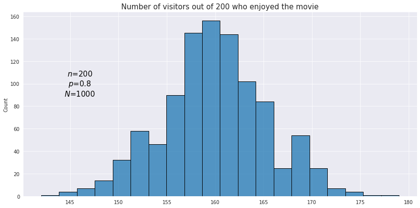
<p>In order to achieve better accuracy with binomial distribution testing the whole experiment may be performed multiple times (or the observations may be resampled with replacement). For example we want to estimate how well the audience likes a new movie. The outcome for each individual cinema visitor is viewed as a Bernoulli trial while the number of satisfied visitors after a session is the result of a single binomial test. Since this measure itself may depend on many factors the results after each session may be quite different. In order to understand the average percentage of the audience satisfaction it may be useful to visualize with a histogram the total number of outcomes for the binomial tests across all sessions. Below is a plot displaying distribution of binomial test
results for 1000 sessions each containing 200 visitors.</p>

<p><img src="/assets/images/probability/binomial_distribution.png" alt="" class="align-center" /></p>

<p>If the number of experiments is reasonably high (specifically, if both $np$ and $n(1−p)$ are greater than 5), the binomial distribution may be closely approximated by the <a href="/probability%20&amp;%20statistics/normal-distribution/">normal distribution</a>. As shown in the image above, the resulting values of a binomial experiment will be concentrated around a certain central value, demonstrating a behavior similar to that of a normal distribution.</p>

<div id="poisson_distribution" />

<h3 id="poisson-distribution">Poisson Distribution</h3>

<p>This distribution is used to model the number of events which occur during a fixed period of time, for example the number of customer complaints per month or the number of trains arriving during a certain hour. Similarly to the binomial distribution, all occurrences of events are considered random and independent, so the occurrence of one event does not affect the probability of another event.</p>

<p>The probability mass function of the Poisson distribution uses prior knowledge of the average number of occurrences per period - parameter $\lambda$. This parameter can actually be derived from the binomial distribution as $\lambda = np$, where $p$ is the probability of a single event occurrence, and $n$ is the number of Bernoulli trials. Both mean and variance of a random variable which follows the Poisson distribution are equal to $\lambda$, and this is the formula of its PMF:</p>

\[f(x; \lambda) = \frac{\lambda^{x}e^{-\lambda}}{x!}\]

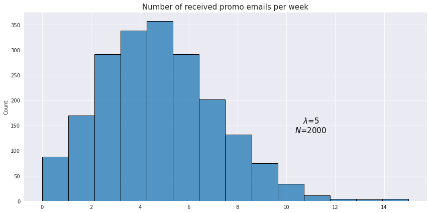
<p>For example, a person receives on average 5 promotional emails from different sellers. The probability of receiving 3 emails would be</p>

\[f(3; 5) = \frac{5^{3}e^{-5}}{3!} \approx 0.14\]

<p>Here is an example of an observed distribution of the number of received emails for a sample of 2000 users.</p>

<p><img src="/assets/images/probability/poisson_distribution.png" alt="" class="align-center" /></p>

<div id="geometric_distribution" />

<h3 id="geometric-distribution">Geometric distribution</h3>

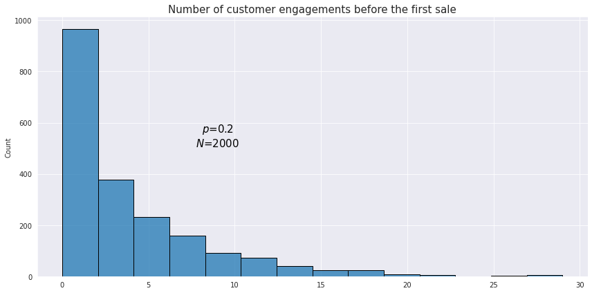
<p>This is a type of distribution which is used to model the number of failures in sequences of Bernoulli trials before the first success (or vice versa). For example we want to know how many customers a retail shop has to engage with before the first sale is made.</p>

<p>The PMF of the geometric distribution is given by the following formula:</p>

\[f(x) = (1-p)^{x} p\]

<p>The formula is pretty intuitive as it just calculates the joint probability of $x$ failures in Bernoulli trials, each having probability of $(1-p)$, and 1 success probability of which is $p$.</p>

<p>Below is an example of what an observed geometric distribution could look like:</p>

<p><img src="/assets/images/probability/geometric_distribution.png" alt="" class="align-center" /></p>

<p>From our example above the probability of having the first successful sale after 2 unsuccessful customer engagements would be</p>

\[f(2) = (1-0.2)^{2} \cdot 0.2 = 0.128\]

<p>The mean of the geometric distribution is defined as $\frac{1-p}{p}$.</p>

<div id="negative_binomial_distribution" />

<h3 id="negative-binomial-distribution">Negative binomial distribution</h3>

<p>This distribution is the generalization of the geometric distribution which is used to model the number of failures before the $n$th success. The PMF is the following:</p>

\[f(x; r) = \binom{x+r-1}{r-1}(1-p)^{x}p^r\]

<p>where $r$ is the required number of successes, $p$ is the probability of a success in a single Bernoulli experiment.</p>

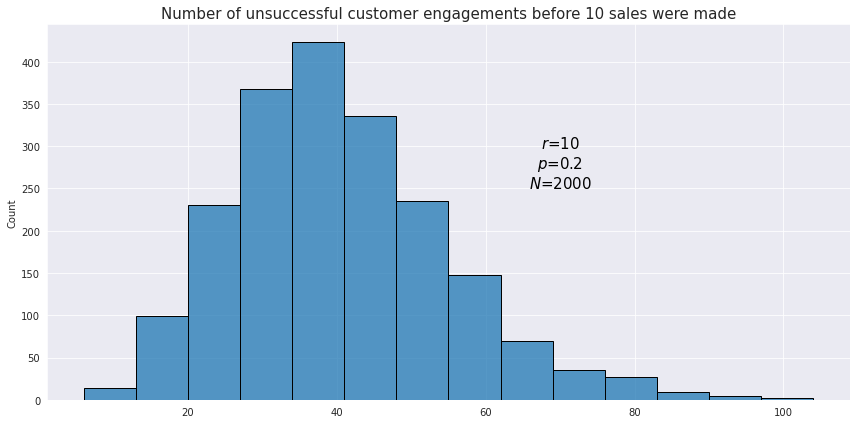
<p>Using the same example as with the geometric distribution, let’s see how the distribution looks like for the number of unsuccessful customer engagements before 10 sales were made.</p>

<p><img src="/assets/images/probability/negative_binomial_distribution.png" alt="" class="align-center" /></p>

<p>The mean of the negative binomial distribution is defined as $\frac{r(1-p)}{p}$, and the variance is $\frac{r(1-p)}{p^2}$.</p>

<h4 id="negative-binomial-as-generalization-over-poisson-distribution">Negative Binomial as Generalization over Poisson Distribution</h4>

<p>The negative binomial distribution is, in fact, often used as a generalization of the Poisson distribution to handle a specific and common issue in count data called overdispersion. Overdispersion occurs when the variance of the data is greater than its mean.</p>

<p>The Poisson distribution makes a strong assumption: its mean is equal to its variance. This works well if events are truly random and independent. However, in real-world data like the number of crashes per device device, the variance is often larger than the mean. This might happen if certain factors (like a specific software bug, heavy usage, or a particular device model) cause some devices to be much more prone to crashing than others. This “extra” variability is not accounted for by the Poisson model.</p>

<p>The negative binomial distribution addresses this by including an extra parameter $\alpha$ that allows the variance to be greater than the mean. It is a more flexible model that can capture this additional, unobserved variability. In order to do that the parametrization of the distribution model needs to shift from $r$ and $p$ to more intuitive $\mu$ and $\sigma$.</p>

<p>In an alternative parametrization model the mean represents the average number of events (e.g., crashes per hour).</p>

<p>The variance is given by:</p>

\[\sigma=\mu + \alpha \mu^2\]

<p>where $\alpha$ is a dispersion parameter that quantifies the overdispersion. When $\alpha$ approaches zero, the negative binomial distribution’s variance approaches its mean, and its shape converges to that of a Poisson distribution.</p>

<h4 id="derivation-of-the-alternative-negative-binomial-distribution-parametrization">Derivation of the Alternative Negative Binomial Distribution Parametrization</h4>

<p>Using the definition of the mean:</p>

\[\frac{1-p}{p} = \frac{\mu}{r}\]

<p>Then putting this into the variance formula:</p>

\[\sigma^2 = \frac{r(1-p)}{p^2} = \frac{r(1-p)}{p} \times \frac{1}{p} = \mu \times \frac{1}{p}\]

<p>This gives us the variance in terms of the mean and the probability of success. Now, let’s use the first equation again to express $p$ in terms of $\mu$ and $r$:</p>

\[1- p = \frac{\mu p}{r}\]

\[1 = p + \frac{\mu p}{r} = p(1+\frac{\mu}{r})\]

\[p = \frac{1}{1+\frac{\mu}{r}}\]

<p>Finally, substitute this expression for p back into the variance formula:</p>

\[\sigma^2 = \mu \times (1+ \frac{\mu}{r}) = \mu + \frac{\mu^2}{r}\]

<p>So $\alpha$ is actually $\frac{1}{r}$.</p>

<div id="uniform_distribution" />

<h3 id="uniform-distribution">Uniform Distribution</h3>

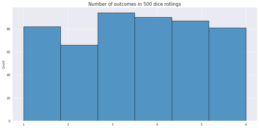
<p>This type of distribution describes processes where every possible outcome has the same chance of occurring. It could be either discrete of continuous. An example of a discrete uniform distribution is rolling of a dice once and expecting any of the possible 6 values.</p>

<p><img src="/assets/images/probability/uniform_distribution.png" alt="" class="align-center" /></p>

<p>The PMF for the discrete distribution is just $\frac{1}{n}$, where $n$ is the number of partitions with the equal probability.</p>

<p>For the continuous distributions the PDF is a constant line:</p>

\[f(x) = \frac{1}{b-a}\]

<p>where $a$ and $b$ are the borders of the distribution.</p>

<p>The expected value of the uniform distribution is defined as the center of the range over which the value is distributed $\frac{a+b}{2}$.</p>

<h2 id="common-continuous-distributions">Common Continuous Distributions</h2>

<h3 id="normal-distribution">Normal Distribution</h3>

<p>Normal distribution, also known as the Gaussian distribution, is arguably the most important and widely used distribution in statistics. It is characterized by its symmetric, bell-shaped curve. Many natural phenomena follow this pattern, such as the height of people, blood pressure, and test scores. The normal distribution is completely defined by its mean ($\mu$) and standard deviation ($\sigma$). Since this is a foundational distibution, it has its own dedicated <a href="/probability%20&amp;%20statistics/normal-distribution/">page</a>.</p>

<div id="student_distribution" />

<h3 id="students-t-distribution">Student’s t-Distribution</h3>

<p>The Student’s t-distribution is a continuous probability distribution that is very similar in shape to the <a href="/probability%20&amp;%20statistics/normal-distribution/">normal distribution</a>. However, it is specifically designed for situations where the sample size is small and the population standard deviation is unknown. Its most distinguishing feature is its fatter tails, which account for the greater uncertainty that comes from working with a small sample of data.</p>

<p>Unlike the normal distribution, which has a constant shape, the shape of the t-distribution changes based on a single parameter: the <a href="/probability/degrees-of-freedom/">degrees of freedom</a> ($\nu$).</p>

<h4 id="properties-of-students-t-distribution">Properties of Student’s t-Distribution</h4>

<ul>
  <li>
    <p><strong>Degrees of Freedom</strong> ($\nu$): This parameter is directly related to the sample size ($n$). The degrees of freedom are calculated as $n$−1.</p>
  </li>
  <li>
    <p><strong>Fatter Tails</strong>: The “fatter tails” mean that the t-distribution assigns a higher probability to extreme values compared to the normal distribution. This reflects the reality that with a small sample, you are more likely to encounter an extreme value by chance.</p>
  </li>
</ul>

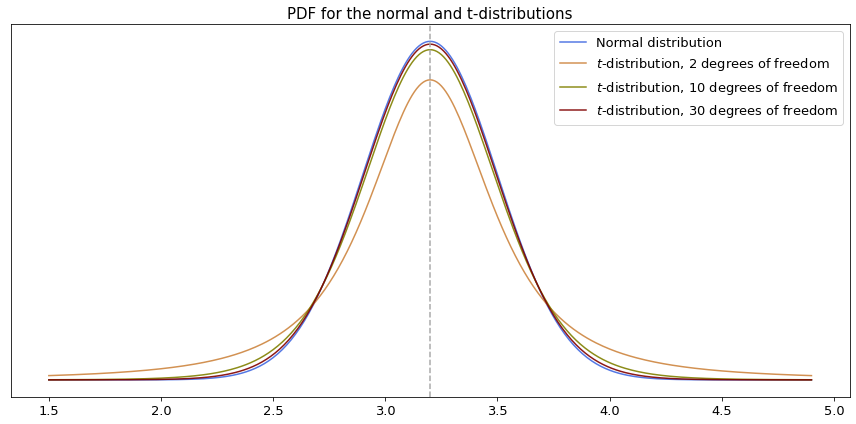
<p>The key property of this distribution is its relationship with the normal distribution. As the degrees of freedom increase (i.e., as the sample size grows), the t-distribution’s shape becomes virtually identical to the standard normal distribution.</p>

<p><img src="/assets/images/probability/normal_and_t_distributions.png" alt="" class="align-center" /></p>

<p>As the size of the sample (and therefore the degrees of freedom) increases, the t-distribution becomes virtually identical to the normal distribution. For a sample size of roughly 30 or more, the two distributions are so close that they can be used interchangeably.</p>

<h4 id="why-is-students-t-distribution-so-important">Why Is Student’s t-Distribution So Important?</h4>

<p>The t-distribution is a cornerstone of inferential statistics because it provides a reliable method for analyzing data from small samples.</p>

<p>Its primary use is in:</p>

<ul>
  <li>
    <p><strong><a href="/probability/hypothesis-testing/">Hypothesis Testing</a></strong>: It is used in the t-test to determine if the means of two groups are significantly different from each other when the sample size is small and the population variance is unknown.</p>
  </li>
  <li>
    <p><strong>Confidence Intervals</strong>: It is used to construct confidence intervals for a population mean using <a href="/probability%20&amp;%20statistics/statistical-inference/">inferential statistics</a>. This allows us to estimate a range of plausible values for the true population mean based on a small sample.</p>
  </li>
</ul>

<p>In essence, while the normal distribution is the “ideal” model for a large population, the t-distribution is the practical and more robust tool for when we have limited data.</p>

<p>Similar to how z-scores and z-tables are used for the <a href="/probability%20&amp;%20statistics/normal-distribution/">normal distribution</a>, the t-distribution has its own tables of precomputed values for different levels of degrees of freedom. This is incredibly useful for practical applications, as it means there is no need to perform complex <a href="/calculus/integrals/">integration</a> over its probability density function when calculating probabilities.</p>

<div id="chi_distribution" />

<h3 id="chi-squared-distribution">Chi-squared distribution</h3>

<p>In a nutshell the chi-square distribution is the distribution of sum of squared values sampled from a <a href="/probability%20&amp;%20statistics/normal-distribution/">normally distributed variable</a>.</p>

\[\chi_k^{2} = \sum_{i=1}^k Z_i^2\]

<p>where $Z_i$ is a randomly drawn value from a normal distribution, and $k$ is the number of <a href="/probability/degrees-of-freedom/">degrees of freedom</a>, which is also equal to the number of drawn values.</p>

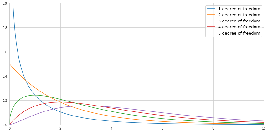
<p>Below is a visualization of the probability density function of the chi-square distribution for a different number of degrees of freedom if the values are drawn from the normal distribution with the mean value 0, and the standard deviation 1.</p>

<p><img src="/assets/images/probability/chi_squared_distributions.png" alt="" class="align-center" /></p>

<p>Notice that since we are squaring the values there are no negative values in the chi-square distribution. If we draw only one value, then there is a high probability that this value is close to 0, since the normal distribution is centered around 0. Therefore the shape of the PDF of chi-square distribution with 1 degree of freedom is heavily skewed towards zero, while the probability of getting bigger numbers becomes minuscule. If we draw more and more numbers increasing the number of degrees of freedom, the sum of squared values causes the center of the PDF of chi-square distribution to be shifted to the right.</p>

<div id="beta_distribution" />

<h3 id="beta-distribution">Beta Distribution</h3>

<p>This distribution is an extension of the negative binomial distribution to the continuous variables. However, instead of modeling the number of successes (or failures), it is used for modeling the distribution of probability.</p>

<p>Let’s imagine that out of 100 customers who went to a gym trial, only 63 decided to buy an annual membership. How would one describe the probability of purchasing a gym membership after trying a trial? The most obvious answer would be say 63%, and this is not wrong, yet it might be useful to resort to a distribution instead of picking just one number for probability. See, 63% is the statistic of a sample, and the true percentage might be different. As such, we might want to know the probability that the true probability of buying a gym membership is greater than 50% for example. This is where the beta distribution comes to rescue because using its probability density function we can simply integrate over all its values higher than 0.5.</p>

<p>The beta distribution is defined for the inclusive range between 0 and 1, and its PDF looks like this:</p>

\[f(x; \alpha, \beta) = \frac{x^{\alpha -1}(1-x)^{\beta -1}}{\mathrm{B}(\alpha, \beta)}\]

<p>where $\alpha$ and $\beta$ reflect the proportion of successes and failures accordingly, and $\mathrm{B}(\alpha, \beta)$ is a normalization coefficient defined as follows:</p>

\[\mathrm{B}(\alpha, \beta) = \frac{\Gamma(\alpha)\Gamma(\beta)}{\Gamma(\alpha+\beta)}\]

<p>The gamma-function $\Gamma$ is an extension of the factorial expression to complex numbers which makes it possible to use it for a continuous range of numbers.</p>

\[\Gamma (n) = (n-1)! = \int_{0}^{\infty} x^{n-1}e^{-x} dx \text{ for } n &gt; 0\]

<p>Now, when we look at the formula of the PDF of the distribution more closely, we can see that it is very similar to the PMF of the negative binomial distribution. Since the beta distribution is continuous, the binomial coefficient from the binomial distribution is replaced with the expression which consists of the gamma functions:</p>

\[\binom {n}{k} = \frac {n!}{k!(n-k)!} = \frac{\Gamma(n+1)}{\Gamma(k+1)\Gamma(n-k+1)} = \frac{1}{\mathrm{B}(k+1, n-k+1)}\]

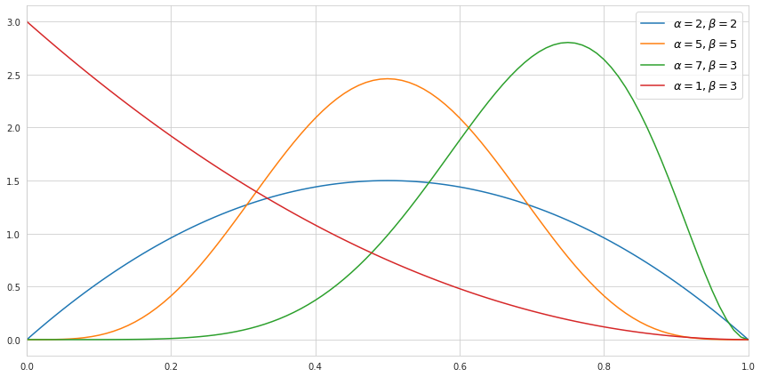
<p>Below we can see how the probability density function of the beta distribution would look like depending on the choice of the parameters.</p>

<p><img src="/assets/images/probability/beta_distribution.png" alt="" class="align-center" /></p>

<p>It is worth mentioning that the higher the value of the parameters - the tighter the values are centered around its mean, which reflects the certainty about the distribution.</p>

<p>The mean of the beta distribution is defined as $\frac{\alpha}{(\alpha+\beta)}$, and the variance is $\frac{\alpha\beta}{(\alpha+\beta)^2(\alpha+\beta+1)}$.</p>

<div id="exponential_distribution" />

<h3 id="exponential-distribution">Exponential Distribution</h3>

<p>This is a continuous distribution which is closely related to the Poisson distribution as it models the time between random independent events. It may also be viewed as a continuous analogue of the geometric distribution. The PDF of the distribution is calculated as follows:</p>

\[f(x; \lambda) = \lambda e^{-\lambda x}\]

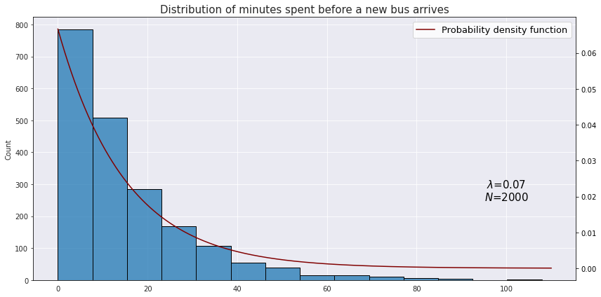
<p>Suppose we would like to model the time between arrival of two buses at some station when on average there are 4 incoming buses for an hour. Translating this into minutes we have $\lambda = \frac{4}{60} \approx 0.07$. This is what a hypothetical distribution of time in minutes would look like:</p>

<p><img src="/assets/images/probability/exponential_distribution.png" alt="" class="align-center" /></p>

<p>The mean of the exponential distribution is $\frac{1}{\lambda}$, and the variance is $\frac{1}{\lambda^2}$.</p>

<div id="weibull_distribution" />

<h3 id="weibull-distribution">Weibull Distribution</h3>

<p>This distribution is a cornerstone of <a href="/survival%20analysis/survival-analysis/">survival analysis</a>,  specifically within the framework of <a href="/survival%20analysis/parametric-survival-models/">parametric survival models</a>.</p>

<p>While the Exponential distribution assumes a constant rate of events (constant hazard, in survival analysis terminology), the Weibull distribution relaxes this assumption by adding a parameter that allows the risk to change over time. This flexibility better reflects the real world, where organisms age, machines wear out, and biological systems adapt.</p>

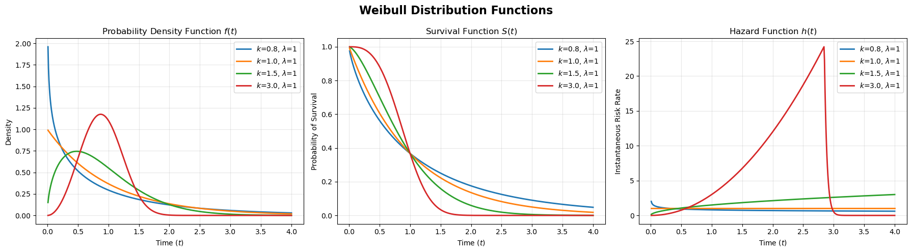
<p><strong>The Shape Parameter $k$</strong> dictates the behavior of the hazard.</p>

<ul>
  <li>$k&lt;1$ (Decreasing Hazard): The risk is high at the start and drops over time. For example in post-surgery survival the highest risk is immediately after the operation: if you survive the first week, your chances of long-term survival improve significantly.</li>
  <li>$k=1$ (Constant Hazard): The risk never changes. In this case the Weibull distribution mathematically transforms into the Exponential distribution.</li>
  <li>$k&gt;1$ (Increasing Hazard): The risk starts low and grows over time. For example a car tire works fine when new, but as miles accumulate, the probability of a blowout increases.</li>
</ul>

<p><strong>The Scale Parameter $\lambda$</strong> stretches or shrinks the curve along the time axis, affecting the time scale of the event (e.g., days vs. years).</p>

<p>The probability density function (PDF) is given by:</p>

\[f(t) = \frac{k}{\lambda}\left(\frac{t}{\lambda}\right)^{k-1}e^{-(t/\lambda)^k}\]

<p>We can better understand this equation by viewing it through the lens of the fundamental survival relationship, where the density is the product of the hazard and the survival function, $f(t) = h(t) S(t)$.</p>

<ul>
  <li>
    <p>The term $e^{-(t/\lambda)^k}$ is the survival function $S(t)$. As $t$ increases, this term decays to 0, representing the probability of survival decreasing over time.</p>
  </li>
  <li>
    <p>The term $\frac{k}{\lambda}\left(\frac{t}{\lambda}\right)^{k-1}$ is the hazard function $h(t)$. This term controls the “instantaneous risk”. For example, if $k=2$ the hazard grows linearly with time, and if $k=1$ the hazard becomes constant.</p>
  </li>
</ul>

<p><img src="/assets/images/probability/Weibull.png" alt="" class="align-center" /></p>

<div id="log_normal_distribution" />

<h3 id="log-normal-distribution">Log-Normal Distribution</h3>

<p>This distribution arises when the logarithm of a random variable is <a href="/probability%20&amp;%20statistics/normal-distribution/">normally</a> distributed.</p>

\[X = e^{\mu + \sigma Z}\]

<p>While the normal distribution results from adding independent random events (the additive Central Limit Theorem), the log-normal distribution results from the multiplication of many independent random effects.</p>

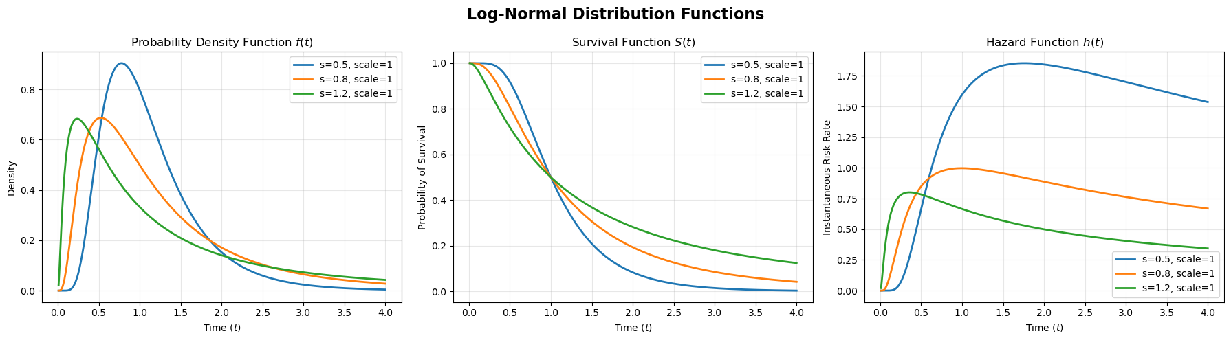
<p>Similar to the normal distribution, the parameters of the log-normal distribution are $\mu$ and $\sigma$, but they refer to the underlying logged data:</p>

<ul>
  <li>
    <p>$\mu$ is the mean of the logged data ($\ln T$). It functions as a scale parameter: if $\mu$ increases, the entire curve shifts to the right.</p>
  </li>
  <li>
    <p>$\sigma$ is the standard deviation of the logged data. This parameter controls the shape (skewness). A higher $\sigma$ results in a much heavier, longer tail to the right, indicating a higher probability of extreme outliers.</p>
  </li>
</ul>

<p><img src="/assets/images/probability/Log-Normal.png" alt="" class="align-center" /></p>

<p>This distribution is used in <a href="/survival%20analysis/survival-analysis/">survival analysis</a> to model the hazard rate which increases in time up to a certain point, and then becomes smaller. For example the risk of dying immediately after a surgery is small, but then rises quickly to a peak (complications usually happen here), and if you survive that peak, your risk drops the longer you live.</p>

<div id="log_logistic_distribution" />

<h3 id="log-logistic-distribution">Log-Logistic Distribution</h3>

<p>The Log-Logistic distribution is the “cousin” of the Log-Normal. To the naked eye, their density plots look almost identical (both are right-skewed humps), but the Log-Logistic has heavier tails (more outliers).</p>

<p>Mathematically, it is the distribution of a variable $T$ whose logarithm follows a Logistic distribution. The Standard Logistic distribution is very similar to the standard <a href="/probability%20&amp;%20statistics/normal-distribution/">normal distribution</a>, but, again, with heavier tails.</p>

<p>Recall the cumulative distribution function (CDF) of a standard logistic variable $z$ (from <a href="/classification/logistic-regresion/">logistic regression</a>):</p>

\[F(t) = \frac{1}{1+e^{-t}}\]

<p>The <a href="/calculus/derivatives/">derivative</a> gives the probability density function:</p>

\[f(t) = \frac{e^{-t}}{(1+e^{-t})^2}\]

<p>We can define $Y= \ln(T)$ which follows a logistic distribution with location parameter $\mu$ (often mapped to $\ln(\alpha)$) and scale parameter $s$ (often mapped to $1/\beta$). Solving it for $T$ creates as log-logistic distribution, and this is how its PDF looks like when parametrized via $\alpha$ and $\beta$:</p>

\[f(t) = \frac{(\beta/\alpha)(t/\alpha)^{\beta-1}}{(1+(t/\alpha)^\beta)^2}\]

<p>In the context of <a href="/survival%20analysis/survival-analysis/">survival analysis</a>, we can break this down into the survival function and the hazard function:</p>

\[S(t)=\frac{1}{1+(t/\alpha)^\beta}\]

\[h(t)=\frac{(\beta/\alpha)(t/\alpha)^{\beta-1}}{1+(t/\alpha)^\beta}\]

<p>The numerator of the hazard function resembles the Weibull hazard. It pulls the risk up (if $\beta&gt;1$). However, the denominator ($1+(t/\alpha)^\beta$) grows faster than the numerator as $t$ gets very large. This forces the hazard to eventually turn around and decrease, creating a “hump” shape similar to the Log-Normal distribution.</p>

<p><img src="/assets/images/probability/Log-Logistic.png" alt="" class="align-center" /></p>]]></content><author><name>Vladyslav Zahorui</name></author><category term="Probability &amp; Statistics" /><category term="probability-distribution" /><category term="probability" /><category term="normal-distribution" /><category term="statistics" /><category term="t-distribution" /><category term="student-distribution" /><category term="probability-mass-function" /><category term="PMF" /><category term="probability-density-function" /><category term="PDF" /><category term="chi-square-distribution" /><category term="binomial-distribution" /><category term="Bernoulli-trial" /><category term="geometric-distribution" /><category term="exponential-distribution" /><category term="poisson-distribution" /><category term="uniform-distribution" /><category term="negative-binomial-distribution" /><category term="beta-distribution" /><category term="gamma-function" /><category term="Gaussian-distribution" /><category term="Weibull-distribution" /><category term="log-normal-distribution" /><category term="log-logistic-distribution" /><summary type="html"><![CDATA[A probability distribution is a function that describes the likelihood of a random variable taking on certain values. Think of it as a model or blueprint for a dataset, showing us the probable outcomes of a random process.]]></summary></entry><entry><title type="html">Survival Analysis</title><link href="https://vzahorui.github.io/survival%20analysis/survival-analysis/" rel="alternate" type="text/html" title="Survival Analysis" /><published>2025-10-06T00:00:00+00:00</published><updated>2025-10-06T00:00:00+00:00</updated><id>https://vzahorui.github.io/survival%20analysis/survival-analysis</id><content type="html" xml:base="https://vzahorui.github.io/survival%20analysis/survival-analysis/"><![CDATA[<p>Survival Analysis, also known as Time-to-Event Analysis, is a specialized branch of <a href="/probability%20&amp;%20statistics/probability-statistics/">statistics</a> focused on analyzing the time until an event of interest occurs.</p>

<p>While it originated in medical research — modeling how long patients survive after treatment — today it spans a wide range of applications:</p>

<ul>
  <li>Medicine: Time until disease recurrence or recovery.</li>
  <li>Engineering: Time until component failure.</li>
  <li>Economics: Duration of unemployment.</li>
  <li>Finance and Business: Time until customer churn or loan default.</li>
</ul>

<p>What distinguishes survival analysis from ordinary regression is its explicit treatment of censoring — the fact that for many observations, the exact event time is not fully observed.</p>

<h2 id="key-concepts-in-survival-analysis">Key Concepts in Survival Analysis</h2>

<p>Three fundamental elements define any survival problem:</p>

<ol>
  <li>The Event (Failure or Hazard)</li>
</ol>

<p>The event is the outcome of interest—the “failure” being studied. It must be clearly defined. Despite the common terminology, the event not necessarily should mean something bad.</p>

<ul>
  <li>In Medicine: Death, recurrence of disease, recovery.</li>
  <li>In Engineering: Failure of a component, equipment breakdown.</li>
  <li>In Business: Customer canceling a subscription, default on a loan.</li>
</ul>

<ol>
  <li>The Time Variable</li>
</ol>

<p>This is the duration from a defined starting point (e.g., date of treatment, product installation, purchase date) until the event occurs. Time is always positive and continuous.</p>

<p>Crucially, in experiments involving multiple subjects, while they may have vastly different absolute start times (e.g., different calendar dates of enrollment), the analysis normalizes them. The clock is effectively reset for each subject, and the variable used in the models is the relative duration (time elapsed) from their individual starting point to the event. This ensures that the focus remains solely on the duration of survival or exposure, rather than the calendar date.</p>

<ol>
  <li>Censoring: The Unique Challenge</li>
</ol>

<p>Censoring occurs when we do not observe the event for a subject during the study period. This is the central mathematical challenge in survival analysis, as standard methods cannot simply ignore or discard these incomplete observations.</p>

<p>The most common type is Right Censoring:</p>

<ul>
  <li>Loss to Follow-up: A patient leaves the study before the event occurs.</li>
  <li>Study Termination: The study concludes before the event occurs for some subjects.</li>
</ul>

<p>For a Right-censored observation, we know the event time is greater than the recorded observation time ($T$&gt;$t$), but we don’t know the exact time of failure. Survival analysis methods are specifically designed to incorporate this partial information.</p>

<p>On the contrary, Left-censoring occurs when we know that the event time is less than the recorded observation time ($T$&lt;$t$).</p>

<p>There is also a type of censoring known as Interval censoring where we know that the event time is between two values.</p>

<h3 id="truncation-in-the-data">Truncation in the Data</h3>

<p>While censoring deals with incomplete event times within the study duration, truncation deals with bias in the selection of subjects for the study itself. A truncated observation is one where the subject is only included in the analysis if their observed event time $T$ falls within a specified window.</p>

<p>The most common form is Left Truncation:</p>

<p>A subject is only observed (and enters the risk set) if their event has not yet occurred by a certain time $L$ (the entry time). In other words, for a subject to be included, their true event time $T$ must be greater than their time of entry $L$ ($T \geq L$).</p>

<p><strong>Example</strong>: Studying the progression of a chronic disease where the disease onset occurred 10 years ago. A subject is only recruited if they have survived for at least 10 years. If a person died 5 years after the disease onset, they would be “left truncated” from the study, leading to a sample that inherently appears healthier (has longer survival times) than the true population.</p>

<p>Survival analysis models must explicitly account for truncation to prevent biased estimation of the survival function and hazard rates.</p>

<h2 id="core-mathematical-functions">Core Mathematical Functions</h2>

<p>Survival analysis is built around several core functions that describe the probabilistic behavior of the time-to-event variable $T$.</p>

<p>The relationships described below are fundamental: knowing any one of $S(t)$, $h(t)$, $f(t)$ allows you to compute the others.</p>

<h3 id="the-survival-function">The Survival Function</h3>

\[S(t)=P(T&gt;t)\]

<p>It gives the probability that the event has not yet occurred by time $t$.</p>

<p>$S(t)$ is always monotonically decreasing, starting at $S(0)=1$ (everyone survives at time zero) and approaching 0 as $t \rightarrow \infty$.</p>

<h3 id="the-density-function">The Density Function</h3>

<p>The event time also has a <a href="/probability%20&amp;%20statistics/statistical-distributions/">probability density function (PDF)</a>, $f(t)$, which represents the probability density of the event occurring at time $t$.</p>

\[f(t) = \lim_{\Delta t \rightarrow 0} \frac{P(t \leq T &lt; t + \Delta t)}{\Delta t}\]

<p><strong>Connection to the Survival Function</strong>: The slope of a survival function is always negative; a steeper negative slope means a faster decrease in survival and thus a higher probability density of the event. Therefore, the density function can be expressed as the negative <a href="/calculus/derivatives/">derivative</a> of the survival function with respect to time.</p>

\[f(t) = - \frac{dS(t)}{dt} = \frac{d}{dt}(1-S(t))\]

<p>The Cumulative Distribution Function (CDF), $F(t)$, is the complement of the survival function. It represents the probability that the event has occurred by time $t$ ($P(T \leq t)$) and can be obtained by <a href="/calculus/integrals/">integrating</a> the density function from 0 to $t$.</p>

\[F(t) = \int_0^t f(t) = \int_0^t \frac{d}{dt}(1-S(t)) = 1 - S(t)\]

<h3 id="the-hazard-function">The Hazard Function</h3>

<p>The hazard function, $h(t)$, is the instantaneous rate of the event occurring at time $t$, given that the individual has survived up to time $t$.</p>

\[h(t)= \lim_{\Delta t \rightarrow 0} \frac{P(t &lt; T \leq t + \Delta t| T &gt; t)}{\Delta t}​\]

<p>The hazard function can increase, decrease, or remain constant over time, reflecting how the risk changes (e.g., risk of infant mortality decreases over time, while risk of many chronic diseases increases with age).</p>

<p>The hazard function is an instantaneous rate based on a conditional probability. By definition $P(A \mid B)=\frac{P(A\cap B)}{P(B)}​$. We can view $A$ as the event occurring in the small interval $[t, t+\Delta t)$ and $B$ as survival up to $t$. $P(A\cap B)$ is $P(A)$, as $A$ implies $B$ (you must survive to time $t$ to have the event at time $t$).</p>

<p>This simplifies to:</p>

\[h(t) = \frac{f(t)}{S(t)}\]

<p>Furthermore, since $f(t) = -S’(t)$, we can see that:</p>

\[h(t) = \frac{-S'(t)}{S(t)} = -\frac{d}{dt}\ln S(t)\]

<p>By integrating both sides, we can express the cumulative hazard function, $H(t)$:</p>

\[H(t) = \int_0^t h(u) du= - [ \ln S(t) - \ln S(0) ] = - \ln S(t)\]

<p>Therefore, if you know one of these functions, you can derive the others. For example, $S(t) = e^{-H(t)}$.</p>

<h2 id="classes-of-models-in-survival-analysis">Classes of Models in Survival Analysis</h2>

<p>Different estimators model $S(t)$ and $h(t)$ with different levels of structure.</p>

<table>
  <thead>
    <tr>
      <th style="text-align: center">Approach</th>
      <th style="text-align: center">Parametric Assumption</th>
      <th style="text-align: center">Typical Use</th>
      <th style="text-align: center">Example model</th>
    </tr>
  </thead>
  <tbody>
    <tr>
      <td style="text-align: center">Non-Parametric</td>
      <td style="text-align: center">No assumption on $S(t)$ and $h(t)$</td>
      <td style="text-align: center">Exploratory, baseline estimation</td>
      <td style="text-align: center"><a href="/survival%20analysis/kaplan-meier-estimator/">Kaplan-Meier Estimator</a></td>
    </tr>
    <tr>
      <td style="text-align: center">Semi-Parametric</td>
      <td style="text-align: center">Functional form for covariate effects, but $h_0(t)$ is free</td>
      <td style="text-align: center">Regression analysis of risk factors</td>
      <td style="text-align: center"><a href="/survival%20analysis/cox-proportional-hazards/">Cox Proportional Hazards Model</a></td>
    </tr>
    <tr>
      <td style="text-align: center">Parametric</td>
      <td style="text-align: center">Fully specified distribution (Exponential, Weibull, Log-Logistic, etc.)</td>
      <td style="text-align: center">Forecasting, reliability, extrapolation</td>
      <td style="text-align: center"><a href="/survival%20analysis/parametric-survival-models/">Parametric Survival Models</a></td>
    </tr>
  </tbody>
</table>

<p>Typically, you build a <a href="/survival%20analysis/kaplan-meier-estimator/">Kaplan-Meier Estimator</a> for exploratory analysis. However, for regression analysis, such as determining the impact of different variables on the survival rate and expected useful life, you will have to build either a semi-parametric <a href="/survival%20analysis/cox-proportional-hazards/">Cox Model</a> or a <a href="/survival%20analysis/parametric-survival-models/">fully parametric one</a>. The latter is better if you need to forecast beyond the observable time period.</p>

<p><a href="/supervised%20learning/tree-like-algorithms/">Tree-based models</a> such as random forest and gradient boosting can also be applied for regression analysis. They typically outperform in terms of predictive accuracy within the observable time period because they can capture non-linear relationships and interactions between variables. However, they are not suited for forecasting beyond the observable time window and do not provide the same level of coefficient interpretability.</p>

<h3 id="the-life-tables">The Life Tables</h3>

<p>The Life Table, or Actuarial Method, is an early non-parametric technique based on grouped intervals (e.g., ages, 5-year windows). It summarizes survival in discrete steps rather than at exact event times.</p>

<p>Typical columns include:</p>

<table>
  <thead>
    <tr>
      <th style="text-align: center">Symbol</th>
      <th style="text-align: center">Meaning</th>
      <th style="text-align: center">Formula</th>
    </tr>
  </thead>
  <tbody>
    <tr>
      <td style="text-align: center">$P_x$</td>
      <td style="text-align: center">Number at risk at stage $x$</td>
      <td style="text-align: center">—</td>
    </tr>
    <tr>
      <td style="text-align: center">$D_x$</td>
      <td style="text-align: center">Deaths between $x$ and $x+1$</td>
      <td style="text-align: center">—</td>
    </tr>
    <tr>
      <td style="text-align: center">$q_x$</td>
      <td style="text-align: center">Probability of dying between $x$ and $x+1$</td>
      <td style="text-align: center">$D_x/P_x$</td>
    </tr>
    <tr>
      <td style="text-align: center">$p_x$</td>
      <td style="text-align: center">Probability of surviving one interval</td>
      <td style="text-align: center">$1-q_x$</td>
    </tr>
    <tr>
      <td style="text-align: center">$l_x$</td>
      <td style="text-align: center">Hypothetical survivors at age $x$</td>
      <td style="text-align: center">$l_0 \prod_{i&lt;x}p_i$</td>
    </tr>
    <tr>
      <td style="text-align: center">$d_x$</td>
      <td style="text-align: center">Hypothetical deaths at age $x$</td>
      <td style="text-align: center">$l_x - l_{x+1}$</td>
    </tr>
  </tbody>
</table>

<p>It is still widely used in demography, insurance, and actuarial science.</p>]]></content><author><name>Vladyslav Zahorui</name></author><category term="Survival Analysis" /><category term="statistics" /><category term="probability" /><category term="censoring" /><category term="Kaplan-Meier-Estimator" /><category term="density-function" /><category term="cumulative-distribution-function" /><category term="survival-function" /><category term="hazard-function" /><category term="life-table" /><summary type="html"><![CDATA[Survival Analysis, also known as Time-to-Event Analysis, is a specialized branch of statistics focused on analyzing the time until an event of interest occurs.]]></summary></entry><entry><title type="html">Kaplan-Meier Estimator</title><link href="https://vzahorui.github.io/survival%20analysis/kaplan-meier-estimator/" rel="alternate" type="text/html" title="Kaplan-Meier Estimator" /><published>2025-10-06T00:00:00+00:00</published><updated>2025-10-06T00:00:00+00:00</updated><id>https://vzahorui.github.io/survival%20analysis/kaplan-meier-estimator</id><content type="html" xml:base="https://vzahorui.github.io/survival%20analysis/kaplan-meier-estimator/"><![CDATA[<p>The Kaplan-Meier (KM) Estimator is the standard way to estimate the survival function $S(t)$ from observed data.</p>

<p>It is non-parametric, meaning it makes no assumptions about the shape of the underlying distribution (unlike a <a href="/probability%20&amp;%20statistics/normal-distribution/">Normal</a> or <a href="/probability%20&amp;%20statistics/statistical-distributions/#exponential_distribution">Exponential distribution</a>).</p>

<p>The output of the estimator is the KM curve, which is a step function where the drops occur at observed event times. It naturally incorporates censored data by adjusting the number of “at-risk” individuals at each step.</p>

<p>Kaplan-Meier Estimator is primarily used for descriptive analysis in scope of the <a href="/survival%20analysis/survival-analysis/">survival analysis</a> and comparing survival curves between two or more groups (e.g., treatment A vs. treatment B).</p>

<h2 id="the-survival-function">The Survival Function</h2>

<p>The KM estimate is calculated as a product of conditional survival probabilities at each distinct event time.</p>

\[\hat S(t) = \prod_{t_i \leq t} \left(1-\frac{d_i}{n_i}\right)\]

<p>Where:</p>
<ul>
  <li>$t_i$ is the time of the i-th distinct event.</li>
  <li>$d_i$ is the number of events (failures) observed at time $t_i$.</li>
  <li>$n_i$​ is the number of subjects at risk (alive and under observation) just before time $t_i$.</li>
</ul>

<p>The resulting $\hat S(t)$ is a step function that only changes value at the points where an event occurs.</p>

<p><img src="/assets/images/survival_analysis/kaplan_meier.png" alt="" class="align-center" /></p>

<h2 id="confidence-interval-calculation">Confidence Interval Calculation</h2>

<p>Before calculating the <a href="/probability%20&amp;%20statistics/sampling-distribution/#confidence_interval">Confidence Interval</a> we must have the variance at hand.</p>

<h3 id="calculation-of-the-variance">Calculation of the Variance</h3>

<p>The Kaplan-Meier estimator is a product of probabilities, and calculating the variance of a product is mathematically difficult. To simplify this, we take the natural logarithm. This turns the difficult product into a manageable sum (since the variance of a sum is just the sum of the variances):</p>

\[\ln \hat S(t) = \sum_{t_i \leq t} \ln \left(1- \hat p_i \right)\]

<p>where $\hat p_i$ is ${d_i}/{n_i}$.</p>

<h4 id="step-1-variance-of-the-log-terms">Step 1: Variance of the Log-Terms</h4>

<p>We first need the variance of each individual term in the sum: $\ln(1-\hat p_i)$. Since this is a non-linear transformation of $p_i$​, we approximate its variability using a <a href="/probability%20&amp;%20statistics/delta-method/">Delta Method</a> linearization.</p>

<p>The <a href="/calculus/derivatives/">derivative</a> of $g(p) = \ln(1-\hat p)$ is $g’(p) = \frac{-1}{1-p}$. So applying the Delta method:</p>

\[Var [\ln(1-\hat p_i)] \approx \left[\frac{-1}{1-p_i} \right]^2 Var(\hat p_i) = \frac{1}{(1-p_i)^2}Var(\hat p_i)\]

<p>Recall that $\hat p_i$ is a <a href="/probability%20&amp;%20statistics/statistical-distributions/#binomial_distribution">binomial</a> proportion which is approximated via the <a href="/probability%20&amp;%20statistics/normal-distribution/">normal distribution</a> with variance $Var(\hat p_i)\approx p_i(1-p_i)/n_i$. Substituting this back in:</p>

\[Var [\ln(1-\hat p_i)] \approx \frac{1}{(1-p_i)^2} \cdot \frac{p_i(1-p_i)}{n_i} = \frac{p_i}{n_i (1-p_i)}\]

<p>By replacing back $p_i$ with ${d_i}/{n_i}$ we simplify the expression for the variance of the Log-Survival:</p>

\[Var [\ln(\hat S(t))] \approx \sum_{t_i \leq t} \frac{d_i}{n_i (n_i-d_i)}\]

<h4 id="step-2-back-transformation-to-hat-st">Step 2: Back-Transformation to $\hat S(t)$</h4>

<p>We now have the variance of the logarithm of the survival function, $Var [\ln(\hat S(t))]$. However, our goal is to find the variance of the survival function itself, $Var [\hat S(t)]$.</p>

<p>To return to the original scale, we must invert the logarithm using the exponential function:</p>

\[\hat S(t)= \exp(\ln \hat S(t))\]

<p>Since the exponential function is non-linear, the variance does not transfer directly. We must apply the Delta Method a second time.</p>

<ul>
  <li>Function: $h(u)=e^u$ (where $u=\ln S(t)$)</li>
  <li>Derivative: $h’(u)=e^{u}=S(t)$</li>
</ul>

<p>Applying the Delta Method formula $Var(h(u))≈[h’(u)]^2 Var(u)$:</p>

\[Var[\hat S(t)] \approx S(t)^2 \cdot Var [\ln(\hat S(t))]\]

<p>The finally we obtain the Greenwood’s formula:</p>

\[Var[\hat S(t)] = S(t)^2 \sum_{t_i \leq t} \frac{d_i}{n_i (n_i-d_i)}\]

<h3 id="common-confidence-interval-ci-constructions">Common Confidence Interval (CI) Constructions</h3>

<p>There are multiple ways to calculate the CI.</p>

<h4 id="wald-ci">Wald CI</h4>

<p>Simple, but can give limits outside $[0,1]$:</p>

\[\hat S(t) \pm z_{1-\alpha/2}\sqrt{Var(\hat S(t))}\]

<h4 id="logarithmic-transform-ci">Logarithmic transform CI</h4>

<p>This method is meant to stabilize multiplicative variability.</p>

<p>Let $g(S)=\ln S$. Then $g’(S)=1/S$ and by the Delta method:</p>

\[Var(\ln \hat S(t)) \approx \frac{Var(\hat S(t))}{\hat S(t)^2} = \sum_{t_i \leq t} \frac{d_i}{n_i (n_i-d_i)}\]

<p>Let’s mark this expression as $V(t)$, then a $(1-\alpha)$ CI for $\ln S$ is</p>

\[\ln \hat S(t) \pm z_{1-\alpha/2}\sqrt{V(t)}\]

<p>Back-transform (exponentiate) to get a CI for $S(t)$:</p>

\[[\hat S(t)e^{-z\sqrt{V}}, \hat S(t)e^{+z\sqrt{V}}]\]

<p>where $z = z_{1-\alpha/2}$</p>

<p>This keeps bounds positive and is multiplicative.</p>

<h4 id="loglog-or-complementary-loglog-transform-ci">Log–log (or complementary log–log) transform CI</h4>

<p>This method is widely used, has good small-sample coverage and stays in $[0,1]$.</p>

<p>Here the non-linear transformation for the Delta method is defined as follows:</p>

\[g(S)= \ln \left(- \ln S\right)\]

<p>Note, $g$ is now defined for $0&lt;S&lt;1$.</p>

<p>Then compute derivative:</p>

\[g'(S) = \frac{d}{dS}\ln(-\ln S) = \frac{1}{S \ln S}\]

<p>Apply the <a href="/probability%20&amp;%20statistics/delta-method/">Delta Method</a>:</p>

\[Var(g(\hat S)) \approx [g'(S)]^2 Var(\hat S) = \left(\frac{1}{S \ln S}\right)^2 S^2 V(t) = \frac{V(t)}{(\ln S)^2}\]

<p>Replacing $S$ by $\hat S$ we get the estimated standard error.</p>

\[SE[g(\hat S(t))] = \frac{\sqrt{V(t)}}{|\ln \hat S(t)|}\]

<p>The absolute value of $\ln \hat S(t)$ in the denominator is used to ensure that the standard error is positive. The confidence inteval on $g(S)$:</p>

\[g(\hat S(t)) \pm z \cdot \frac{\sqrt{V(t)}}{|\ln \hat S(t)|}\]

<p>Invert the transform to get a CI for $S(t)$. The inverse function is</p>

\[S=\exp⁡(−\exp⁡(g))\]

<p>Because $S = \exp(-\exp(g))$ is decreasing in $g$, when mapping the two end points you must swap them. The conventional formulas are:</p>

\[\text{Lower CI} = \exp\left[-\exp\left(\ln(-\ln \hat S(t)) + z \cdot \frac{\sqrt{V(t)}}{|\ln \hat S(t)|}\right)\right]\]

\[\text{Upper CI} = \exp\left[-\exp\left(\ln(-\ln \hat S(t)) - z \cdot \frac{\sqrt{V(t)}}{|\ln \hat S(t)|}\right)\right]\]

<h3 id="practical-notes-and-edge-cases">Practical Notes and Edge Cases</h3>

<ul>
  <li>If $\hat S(t)=0$ or $\hat S(t)=1$ exactly, the log or log–log transforms are undefined. In practice you avoid trying to transform at exact 0 or 1 (e.g. report one-sided CIs, or stop at the last time where $\hat S&gt;0$, or use small continuity adjustments).</li>
  <li>The simple Wald CI can produce negative lower bounds or upper bounds &gt;1 — this is why log or log–log transforms are preferred.</li>
  <li>The log–log CI works well especially for moderate sample sizes and when the survival is neither extremely close to 0 nor 1.</li>
</ul>

<h2 id="testing-for-equality-of-two-estimators-log-rank-test">Testing for Equality of two Estimators: Log-Rank Test</h2>

<p>The log-rank test is the natural nonparametric comparison test — it compares observed and expected events at each time using hypergeometric (or approximated binomial) allocation, and sums the standardized differences; it is asymptotically $\chi^2_1$ for two groups.</p>

<p>Compare survival experience of two groups (say group 1 and group 2). <a href="/probability/hypothesis-testing/">Null hypothesis</a>:</p>

\[H_0: \text{hazard functions are equal} (\lambda_1(t) = lambda_2(t) \forall t)\]

<p>or equivalently the survival curves are the same.</p>

<p>At each time event $t_i$:</p>

<ul>
  <li>$n_{1i}, n_{2i}$ be numbers at risk in group 1 and 2 just before $t_i$,</li>
  <li>$n_i = n_{1i}+n_{2i}$,</li>
  <li>$d_{1i}, d_{2i}$ be observed events at $t_i$ in the two groups,</li>
  <li>$d_i = d_{1i} + d_{2i}$.</li>
</ul>

<p>Under $H_0$, given that $d_i$ events happen at time $t_i$ among the $n_i$ at risk, the number assigned to group 1 has a hypergeometric distribution (choose $d_i$ from $n_i$ without replacement). Thus the expected number of events in group 1 at time $t_i$ is:</p>

\[E_{1i} = n_{1i}\frac{d_i}{n_i}\]

<p>and the variance (hypergeometric variance) is:</p>

\[Var(d_{1i}) = \frac{n_{1i} n_{2i}}{n_i^2} \cdot d_{i} \cdot \frac{n_i - d_i}{n_1 - 1}\]

<p>Here is some intuition behind this formula:</p>

<ul>
  <li>$\frac{n_{1i} n_{2i}}{n_i^2}$ is the relative mixing between groups (if one group is small, variance drops).</li>
  <li>$d_i$ is number of total failures — more failures → more randomness in who fails.</li>
  <li>$\frac{n_i - d_i}{n_1 - 1}$ is the finite-population correction: drawing without replacement reduces variability.</li>
</ul>

<p>If $n_i$ is large, the factor $(n_i-d_i)/(n_i-1)$ is close to 1 and the variance approximates the binomial form.</p>

<h3 id="the-log-rank-statistic">The log-rank statistic</h3>

<p>Form the sum of observed minus expected events over all distinct failure times:</p>

\[U = \sum_{t_i} (d_{1i} - E_{1i})\]

<p>Under $H_0$ the mean of $U$ is 0. The variance of $U$ is</p>

\[Var(U) = \sum_{t_i} Var(d_{1i}) = \sum_{t_i} \frac{n_{1i} n_{2i} d_i (n_i - d_i)}{n_i^2(n_1 - 1)}\]

<p>Then we can calculate z-statistic as</p>

\[Z = \frac{U}{\sqrt{Var(U)}}\]

<p>For large samples $Z\approx \mathcal {N}(0,1)$ under $H_0$, so the usual test uses</p>

\[\chi^2 = Z^2 \approx \chi_1^2\]]]></content><author><name>Vladyslav Zahorui</name></author><category term="Survival Analysis" /><category term="survival-analysis" /><category term="survival-function" /><category term="logarithm" /><category term="delta-method" /><category term="derivative" /><summary type="html"><![CDATA[The Kaplan-Meier (KM) Estimator is the standard way to estimate the survival function $S(t)$ from observed data.]]></summary></entry><entry><title type="html">Cox Proportional Hazards Model</title><link href="https://vzahorui.github.io/survival%20analysis/cox-proportional-hazards/" rel="alternate" type="text/html" title="Cox Proportional Hazards Model" /><published>2025-10-06T00:00:00+00:00</published><updated>2025-10-06T00:00:00+00:00</updated><id>https://vzahorui.github.io/survival%20analysis/cox-proportional-hazards</id><content type="html" xml:base="https://vzahorui.github.io/survival%20analysis/cox-proportional-hazards/"><![CDATA[<p>While the <a href="/survival%20analysis/kaplan-meier-estimator/">Kaplan–Meier estimator</a> tells us how <a href="/survival%20analysis/survival-analysis/">survival probability</a> changes over time, it doesn’t explain why — it cannot handle predictors or covariates.</p>

<p>The Cox model answers that question by linking covariates (e.g., age, treatment, income) to the hazard rate, i.e., the instantaneous risk of the event occurring.</p>

<h2 id="the-model-structure">The Model Structure</h2>

<p>The hazard for individual $i$ with covariates $X_i = (X_{i1}, X_{i2}, …, X_{im})$</p>

\[h(t|X_i) = h_0(t)\exp(\beta_1 X_{i1} + \beta_2 X_{i2} + ... + \beta_n X_{im})\]

<p>where:</p>
<ul>
  <li>$h_0(t)$ is the baseline hazard function — unspecified (non-parametric).</li>
  <li>$\exp(\beta_j)$ is the multiplicative effect of covariate $X_j$ on the hazard.</li>
  <li>$\beta_j$ is the log-hazard ratio coefficient.</li>
</ul>

<p>Each covariate $X_k$ multiplies the hazard by a fixed proportion $e^{\beta_k}$.</p>

<p>So, for example if $\beta_k = 0.7$, then one-unit increase in $X_k$ increases the hazard by $e^{0.7} \approx 2.01$ times. And if $\beta_k = -0.7$, for example, then the hazard is multiplied by $e^{-0.7} \approx 0.5$, so it’s effectively halved.</p>

<p>Crucially, this increase/decrease is proportionate, not absolute — it scales the whole hazard curve up or down, keeping its shape over time identical.</p>

<p>The hazard ratio between two individuals $i$ and $j$ with covariate vectors $X_i$ and $X_j$ is:</p>

\[\frac{h(t|X_i)}{h(t|X_j)} = \exp(\beta^{T} (X_i - X_j))\]

<p>Notice how the baseline hazard function disappeared. Importantly, this ratio is independent of time, which is the assumption of proportional hazards model.</p>

<h2 id="partial-likelihood-estimation">Partial Likelihood Estimation</h2>

<p>Unlike parametric models, the Cox model doesn’t specify $h_0(t)$. Yet, we still want to estimate the regression coefficients $\beta$ the effect of covariates on the hazard. The partial likelihood cleverly eliminates $h_0(t)$ by conditioning on the set of individuals who are at risk when an event occurs.</p>

<p>If the ordered event times are $t_{(1)}, t_{(2)}, …, t_{(n)}$, and $R(t_{(k)})$ is the risk set (subjects still under observation just before $t_{(k)}$), the partial likelihood is:</p>

\[L(\beta) = \prod_{k=1}^n \frac{\exp(\beta^T X_{(k)})}{\sum_{j \in R(t_{(k)})} \exp(\beta^T X_{j})}\]

<p>Taking logs gives the partial log-likelihood, which is <a href="/optimization/maximum-likelihood/">maximized</a> to estimate $\hat \beta$.</p>

<p>This method automatically accounts for right-censoring, because censored individuals remain in the risk sets up to their censoring time.</p>

<h2 id="interpretation-of-hazard-ratio">Interpretation of Hazard Ratio</h2>

<p>Each coefficient $\beta_j$ corresponds to a log hazard ratio:</p>

\[HR_j = \exp(\beta_j)\]

\[\ln HR_j = \beta_j\]

<ul>
  <li>$HR_j &gt; 1$: higher risk of the event.</li>
  <li>$HR_j &lt; 1$: protective (lower risk).</li>
  <li>$HR_j = 1$: no effect.</li>
</ul>

<p><a href="/probability%20&amp;%20statistics/sampling-distribution/#confidence_interval">Confidence intervals</a> for $HR_j$ are constructed as:</p>

\[\exp(\beta_j \pm z_{\alpha/2 \text{SE}(\beta_j)})\]

<h2 id="extensions-of-the-cox-model">Extensions of the Cox Model</h2>

<h3 id="stratified-cox-model">Stratified Cox Model</h3>

<p>Used when the baseline hazard differs across subgroups (e.g., men vs. women), but covariate effects are assumed common.</p>

\[h(t|X, \text{stratum}=s) = h_{0s}(t)\exp(\beta^T X)\]

<p>Each stratum has its own $h_{0s}(t)$, but a shared $\beta$. This allows the shape and level of the hazard over time to differ across groups — while keeping the same multiplicative effect of covariates on the hazard within each stratum.</p>

<p>Partial likelihood is constructed per stratum, and then multiplied together:</p>

\[L(\beta) = \prod_{s=1}^S \prod_{k=1}^n \frac{\exp(\beta^T X_{(k)})}{\sum_{j \in R(t_{(k)})} \exp(\beta^T X_{j})}\]

<h3 id="time-dependent-covariates">Time-Dependent Covariates</h3>

<p>Some covariates change over time — e.g., blood pressure, medication status.
These are modeled as $X_i (t)$:</p>

\[h(t|X_i (t)) = h_{0}(t)\exp(\beta^T X)\]

<p>This allows modeling dynamic effects such as the impact of treatment after initiation.</p>

<h3 id="non-proportional-hazards-and-interactions">Non-Proportional Hazards and Interactions</h3>

<p>If the proportionality assumption fails, interactions with time can be added:</p>

\[h(t|X_i (t)) = h_{0}(t)\exp(\beta_1 X + \beta_2 X \cdot g(t))\]

<p>where $g(t)$  might be $\log t$, $t$, or a spline term, allowing covariate effects to vary over time.</p>]]></content><author><name>Vladyslav Zahorui</name></author><category term="Survival Analysis" /><category term="survival-analysis" /><category term="hazard-function" /><category term="log-likelihood" /><category term="partial-likelihood" /><category term="confidence-interval" /><summary type="html"><![CDATA[While the Kaplan–Meier estimator tells us how survival probability changes over time, it doesn’t explain why — it cannot handle predictors or covariates.]]></summary></entry><entry><title type="html">Parametric Survival Models</title><link href="https://vzahorui.github.io/survival%20analysis/parametric-survival-models/" rel="alternate" type="text/html" title="Parametric Survival Models" /><published>2025-10-06T00:00:00+00:00</published><updated>2025-10-06T00:00:00+00:00</updated><id>https://vzahorui.github.io/survival%20analysis/parametric-survival-models</id><content type="html" xml:base="https://vzahorui.github.io/survival%20analysis/parametric-survival-models/"><![CDATA[<p>Parametric survival models assume that survival times follow a known probability distribution.
Unlike non-parametric methods (<a href="/survival%20analysis/kaplan-meier-estimator/">Kaplan–Meier</a>) or semi-parametric ones (<a href="/survival%20analysis/cox-proportional-hazards/">Cox PH</a>), these models specify the exact form of the hazard function $h(t)$.</p>

<p>This yields interpretable parameters, smooth curves, and the ability to predict beyond the observed data range.</p>

<h2 id="model-framework">Model Framework</h2>

<p>A parametric survival model defines a probability density $f(t;\theta)$ and cumulative distribution $F(t;\theta)$ with parameters $\theta$ of the hazard event. The survival and hazard functions are expressed as follows:</p>

\[S(t) = 1 - F(t;\theta)\]

\[h(t) = \frac{f(t; \theta)}{S(t; \theta)}\]

<p>With covariates $X$, the hazard or survival time is related through a regression structure, typically via one of two formulations described below.</p>

<h3 id="proportional-hazards-ph-form">Proportional Hazards (PH) Form</h3>

\[h(t|X) = h_0(t) \exp(\beta^T X)\]

<p>Same structure as the Cox model, but here $h_0(t)$ is known (e.g., <a href="/probability%20&amp;%20statistics/statistical-distributions/#exponential_distribution">exponential</a> or Weibull).</p>

<h3 id="accelerated-failure-time-aft-form">Accelerated Failure Time (AFT) Form</h3>

<p>A subclass of parametric survival models focusing on time scaling rather than hazard scaling. Equivalent to log-linear regression on $T$:</p>

\[\log(T_i) = \mu + \beta^T X_i + \sigma \varepsilon_i\]

<p>where $\varepsilon_i$ follows a known distribution (e.g., extreme value, logistic, normal).
This model describes how covariates accelerate or decelerate the event time.</p>

<p>For example, if $\exp (\beta_j) = 1.5$ then it would mean that the expected survival time is 1.5 longer for a one-unit increase in $X_j$</p>

<h2 id="common-parametric-distributions">Common Parametric Distributions</h2>

<table>
  <thead>
    <tr>
      <th style="text-align: center">Distribution</th>
      <th style="text-align: center">Survival function $S(t)$</th>
      <th style="text-align: center">Hazard function $h(t)$</th>
      <th style="text-align: center">Hazard function shape</th>
      <th style="text-align: center">Interpretation</th>
    </tr>
  </thead>
  <tbody>
    <tr>
      <td style="text-align: center">Exponential</td>
      <td style="text-align: center">$e^{-\lambda t}$</td>
      <td style="text-align: center">$\lambda$</td>
      <td style="text-align: center">Constant</td>
      <td style="text-align: center">Memoryless process</td>
    </tr>
    <tr>
      <td style="text-align: center">Weibull</td>
      <td style="text-align: center">$e^{-(\lambda t)^{k}}$</td>
      <td style="text-align: center">$\lambda k(t)^{k-1}$</td>
      <td style="text-align: center">increases if $k$ &gt; 1, decreases if $k$ &lt; 1</td>
      <td style="text-align: center">Very flexible; includes exponential as $k=1$</td>
    </tr>
    <tr>
      <td style="text-align: center">Log-Logistic</td>
      <td style="text-align: center">$[1+t/ \lambda^{k}]^{-1}$</td>
      <td style="text-align: center">$\frac{(k/\lambda)(t/\lambda)^{k-1}}{1+t/ \lambda^{k}}$</td>
      <td style="text-align: center">Unimodal</td>
      <td style="text-align: center">Hazard rises then falls</td>
    </tr>
    <tr>
      <td style="text-align: center">Log-Normal</td>
      <td style="text-align: center">$1- \Phi\left(\frac{\ln t - \mu}{\sigma} \right)$</td>
      <td style="text-align: center">non-monotonic</td>
      <td style="text-align: center">Flexible</td>
      <td style="text-align: center">Useful when long right tail</td>
    </tr>
  </tbody>
</table>

<p>Each provides a different hazard shape, letting the analyst select based on domain knowledge or data diagnostics.</p>

<h2 id="parameter-estimation">Parameter Estimation</h2>

<p>Parameters are estimated with <a href="/optimization/maximum-likelihood/">Maximum Likelihood Estimation</a>:</p>

\[\mathcal{L}(\theta) = \prod_{i=1}^n [f(t_i; \theta)]^{\delta_i} [S(t_i; \theta)]^{1-\delta_i}\]

<p>where $\delta_i = 1$ if the event occurred, 0 if censored.
This formulation naturally accounts for right-censoring.</p>

<h2 id="parametric-vs-semi-parametric-cox-ph-estimator">Parametric vs Semi-parametric (Cox PH) Estimator</h2>

<table>
  <thead>
    <tr>
      <th style="text-align: center">Feature</th>
      <th style="text-align: center">Cox PH</th>
      <th style="text-align: center">Parametric Model</th>
    </tr>
  </thead>
  <tbody>
    <tr>
      <td style="text-align: center">Baseline hazard $h_0(t)$</td>
      <td style="text-align: center">Unknown, estimated nonparametrically</td>
      <td style="text-align: center">Known functional form (Exponential, Weibull, Log-logistic, etc.)</td>
    </tr>
    <tr>
      <td style="text-align: center">Assumption strength</td>
      <td style="text-align: center">Weak (semi-parametric)</td>
      <td style="text-align: center">Strong</td>
    </tr>
    <tr>
      <td style="text-align: center">Interpretability</td>
      <td style="text-align: center">Relative risk (hazard ratio)</td>
      <td style="text-align: center">Can yield absolute predictions (mean survival time, etc.)</td>
    </tr>
    <tr>
      <td style="text-align: center">Extrapolation</td>
      <td style="text-align: center">Limited (data-driven)</td>
      <td style="text-align: center">Possible (based on assumed distribution)</td>
    </tr>
  </tbody>
</table>

<p>Suppose we use Weibull (parametric) model in PH form:</p>

\[h(t|X) = \lambda k t^{k-1} e^{\beta^T X}\]

<p>Here $\lambda$ and $k$ distribution parameters controlling scale and shape. So it’s also “proportional hazards” (covariates enter multiplicatively), but unlike with Cox PH the shape of the hazard over time is fixed by the Weibull functional form.</p>

<p>On the other hand, the Cox model can fit a much wider range of survival patterns without assuming the exact distribution of survival times which makes it a more robust and flexible choice.</p>

<p>For demonstration purposes let’s fit both models to simulated data to see how they differ. The survival function from parametric Weibull distribution will take the following form</p>

\[S(t|X) = \exp[-(\lambda t)^k e^{\beta^T X}]\]

<p>And the survival function from from Cox semi-parametric model will take this form:</p>

\[S(t|X) = \exp[-(h_0(t) e^{\beta^T X}]\]

<p>We have a single covariate $X$ which can assume values 1 or 0.</p>

<p><img src="/assets/images/survival_analysis/cox_vs_weibull.png" alt="" class="align-center" /></p>

<p>As can be seen from the example plot above, Weibull fit, unlike Cox PH, produces a smooth curve. Even though the fitted distribution is not the same as the one which generates the data, it can still be closer to it because the parameters are considering the change in time.</p>

<table>
  <tbody>
    <tr>
      <td>On the other hand, Cox PH is also pretty close. Even if we consider the case when $X=0$ then the survival function collapses to this: $S(t</td>
      <td>X) = \exp[-(h_0(t)]$ which becomes the average survival regardless of the actual $X$. And this is exactly what we observe on the chart.</td>
    </tr>
  </tbody>
</table>]]></content><author><name>Vladyslav Zahorui</name></author><category term="Survival Analysis" /><category term="survival-analysis" /><category term="survival-function" /><category term="logarithm" /><category term="hazard-function" /><category term="Weibull-distribution" /><category term="maximum-likelihood-estimation" /><category term="accelerated-failure-time" /><summary type="html"><![CDATA[Parametric survival models assume that survival times follow a known probability distribution. Unlike non-parametric methods (Kaplan–Meier) or semi-parametric ones (Cox PH), these models specify the exact form of the hazard function $h(t)$.]]></summary></entry><entry><title type="html">Linear regression</title><link href="https://vzahorui.github.io/regression/linear-regression/" rel="alternate" type="text/html" title="Linear regression" /><published>2025-10-01T00:00:00+00:00</published><updated>2025-10-01T00:00:00+00:00</updated><id>https://vzahorui.github.io/regression/linear-regression</id><content type="html" xml:base="https://vzahorui.github.io/regression/linear-regression/"><![CDATA[<p>Linear regression is the simplest and most widely used form of <a href="/regression/regression-analysis/">regression analysis</a>. It assumes a straight-line relationship between a dependent variable ($Y$) and one or more independent variables ($X$). The primary goal is to find the line that best summarizes the observed data, allowing us to estimate the change in $Y$ associated with a unit change in $X$.</p>

<h2 id="the-pre-modeling-step-correlation">The Pre-Modeling Step: Correlation</h2>

<p>Before fitting any line, the first step in linear regression is confirming that a linear relationship even exists. This is assessed using <a href="/regression/correlation/">covariance and correlation</a>.</p>

<ul>
  <li>Covariance measures how two variables vary together (in the same or opposite direction).</li>
  <li>Correlation is the standardized version of covariance, providing a single number (between −1 and +1) that quantifies the strength and direction of the relationship, independent of the variables’ units.</li>
</ul>

<p>A strong correlation (close to −1 or +1) is a necessary signal that a linear regression model may be appropriate.</p>

<h2 id="the-equation-of-the-line">The Equation of the Line</h2>

<p>Single variable linear regression explains the relationship between single input variable and the output:</p>

\[y = a + bx + \varepsilon\]

<p>where $a$ and $b$ are parameters which explain the behaviour of the dependent variable according to the values of the independent one, and $\varepsilon$ is the residual (or error term).</p>

<p>The general form of linear regression however is the multivariable one where multiple predictors are taken into consideration:</p>

\[y = \beta_0 + \sum_{i=1}^n \beta_i x_i + \varepsilon\]

<p>where $\beta_i$ are the weights of each independent variable.</p>

<p>A key feature of linear regression models is that it is assumed that a certain change in the variables causes proportional change in the output (which is not the case in non-linear models). The output is basically treated as a linear combination of predictors.</p>

<div id="gaussian_noise" />

<h3 id="gaussian-noise">Gaussian noise</h3>

<p>In practice there are always factors which are impossible to explain and predict and which may cause surprisingly different results from those that we expect. Therefore there is always going to be some difference between estimated (predicted) and actually observed values - the residuals, even for the variables which seem to be perfectly correlated.</p>

<p>It is common to view the relationship between two observed variables on a scatterplot. Seeing each individual observation helps to estimate the level of variation of the dependent variable, as well as to identify outliers. Below is an example of a nearly linear relationship between two variables which exhibits a certain amount of variation.</p>

<p><img src="/assets/images/regression/residuals_demo.png" alt="" class="align-center" /></p>

<p>According to the <a href="/probability%20&amp;%20statistics/sampling-distribution/central_limit">Central Limit Theorem</a> if the number of observations is large enough - the residuals have <a href="/probability%20&amp;%20statistics/normal-distribution/">normal distribution</a> with the mean value of 0. This basically means that for a modeled relationship between two or more variables the observed variation is mainly clustered around the estimated values. Since normal distribution is also called Gaussian distribution, the distribution of residuals around estimated values is called Gaussian noise.</p>

<div id="matrix_notation" />

<h2 id="matrix-notation">Matrix notation</h2>

<p>For computation purposes it is better to represent the relationship between the dependent and independent variables with matrix notation:</p>

\[Y = X \beta + \varepsilon\]

<p>where $Y$ is the group of all outputs and $X$ is the composition of all predictors for each particular output:</p>

\[Y = \left[ \begin{array}{c}
y_1 \\
y_2 \\
... \\
y_n
\end{array} \right]
\text{ }
X = \left[ \begin{array}{ccccc}
1 &amp; x_11 &amp; x_12 &amp; ... &amp; x_1n \\
1 &amp; x_21 &amp; x_22 &amp; ... &amp; x_2n \\
... &amp; ... &amp; ... &amp; ... &amp; ... \\
1 &amp; x_n1 &amp; x_n2 &amp; ... &amp; x_nn
\end{array} \right]\]

<p>$\beta$ is the vector of parameters (weights) of each predictor, and $\varepsilon$ is the vector of errors (Gaussian noise). This variable captures all other factors which influence the dependent variable y other than the regressors.</p>

<p>The parameters $\beta$ of such equation are usually estimated with <a href="/regression/linear-least-squares/">least squares</a>, however other methods such as maximum likelihood or robust estimation techniques can be employed.</p>

<div id="confidence_interval_coef" />

<h2 id="confidence-intervals-of-the-coefficients">Confidence intervals of the coefficients</h2>

<p><a href="/probability%20&amp;%20statistics/sampling-distribution/#confidence interval">Recall</a> that the confidence interval from a sample is the region around the sample mean, which with a certain level of confidence contains the true mean.</p>

\[(\bar X - Z \cdot SE; \bar X + Z \cdot SE)\]

<p>where $Z$ is the critical value for a given significance level (confidence level minus 1), and $SE$ is the <a href="/probability%20&amp;%20statistics/sampling-distribution/#sample_mean_variance">standard error</a>.</p>

<p>In case of the linear regression the coefficients are calculated based on sample data so they should be viewed as sample means. The variances of the coefficients may be estimated with the covariance matrix, as described <a href="/regression/correlation/#variance_coefficients">here</a>. Then the standard error can be obtained by dividing them by the square root of the number of observations.</p>

<p>When we are dealing with a sample, and the true variance is unknown, instead of the critical value $Z$, which assumes the <a href="/probability%20&amp;%20statistics/normal-distribution/">normal distribution</a>, the $t$-value from the <a href="/probability%20&amp;%20statistics/statistical-distributions/#student_distribution">$t$-distribution</a> is used. The number of <a href="/probability/degrees-of-freedom/">degrees of freedom</a> for the $t$-value in case of the linear regression is ($n$-$m$-1), where $n$ is the number of observations, and $m$ is the number of independent variables.</p>

<p><a href="#page-title" class="back-to-top">Back to top ↑</a></p>

<div id="other_assumptions" />

<h2 id="other-assumptions">Other assumptions</h2>

<p>Apart from the linear nature of relationship between predictors and the output the linear regression estimation relies on a number of other assumptions:</p>

<ul>
  <li>Absence of perfect multicollinearity among predictors - that is that none of the predictors can be expressed as a copy or a linear combination of other predictors.</li>
  <li>Independence of errors - absence of correlation among errors in different output values.</li>
  <li><a href="/probability%20&amp;%20statistics/normal-distribution/">Normal distribution</a> of the error term with the mean value of 0.</li>
  <li><a href="/regression/heteroscedasticity/">Homoscedasticity</a> - constant variance of the error term regardless of the values of independent variables.</li>
</ul>

<p>If not all of the assumptions are satisfied then the model might not have some of the required variables which explain the behaviour of errors, or instead might have redundant variables causing multicollinearity. Or maybe the relationship among variables is non-linear.</p>

<p>If the errors are correlated and/or heteroscedastic, instead of minimizing the sum of squares ($\varepsilon^{T} \varepsilon$), the following <a href="/optimization/distance-metrics/#mahalanobis_distance">Mahalanobis distance</a> has to be minimized: $\varepsilon^{T}\Omega^{-1}\varepsilon$. Where $\Omega$ is the covariance matrix of the errors, which is not equal to the identity matrix as in the case of homoscedastic independent errors.</p>

<p>Then in order to estimate the parameters, instead of the <a href="/regression/linear-least-squares/">ordinary least squares</a> (OLS) the generalized least squares provides the best estimation by taking into account the covariance of the error term:</p>

\[\beta = (X^{T}\Omega^{-1}X)^{-1}X^{T}\Omega^{-1}Y\]

<p>In practice however, the true covariance matrix is not known so it needs to be estimated from the sample. In this case the method of solving is called feasible generalized least squares (FGLS).
<a href="#page-title" class="back-to-top">Back to top ↑</a></p>

<div id="hypothesis_tests" />

<h2 id="hypothesis-testing-in-linear-regression">Hypothesis testing in linear regression</h2>

<p>In scope of linear regression we may want to test the significance of the model in general, and the significance of each individual parameter.</p>

<div id="significance_of_params" />

<h3 id="significance-of-the-parameters">Significance of the parameters</h3>

<p>When testing the parameters we perform the <a href="/probability/hypothesis-testing/">hypothesis test</a> of whether a given parameter is equal to 0:</p>

<p>    
$H_0: \beta_i = 0$</p>

<p>    
$H_a: \beta_i \ne 0$</p>

<p>So for a given significance level the $t$-statistic is calculated:</p>

<p>    
$t = \frac{\beta_i - 0}{SE_i}$</p>

<p>where $SE_i$ is the <a href="/probability%20&amp;%20statistics/sampling-distribution/#sample_mean_variance">standard error</a> of the $i$th coefficient.</p>

<p>If the resulting $t$-statistic has corresponding $p$-value less than the significance level then the null hypothesis is rejected, and the parameter of the regression is considered significant.
<a href="#page-title" class="back-to-top">Back to top ↑</a></p>

<div id="significance_of_model" />

<h3 id="significance-of-the-model">Significance of the model</h3>

<p>In essence this test checks whether inclusion of independent variables (all at once) makes a better model than the model without independent variables.</p>

<p>The null hypothesis here implies that all of the coefficients at independent variables are equal to 0, and the alternative would mean that at least one of them is not equal to zero. The test statistic in this case would be <a href="/probability/hypothesis-test-parametric-statistics/#mean_more_samples">F-test</a>.</p>

<p>On the whole, there might be cases when the model in general is statistically significant but each individual coefficient is not. This happens when the predictor variables are highly correlated among themselves. Due to multicollinearity the coefficient values become unstable, and their confidence intervals inflated, so these intervals include 0.
<a href="#page-title" class="back-to-top">Back to top ↑</a></p>

<div id="validation" />

<h2 id="validation-of-assumptions">Validation of assumptions</h2>

<p>Linear regression via <a href="/regression/linear-least-squares/">ordinary least squares</a> is safe to apply if all of the assumptions are satisfied. Using the Boston houses prices dataset let’s perform a typical check in order to ascertain whether it is reasonable to apply linear regression to predict prices.</p>

<div id="validation_of_linear" />

<h3 id="linear-relationship">Linear relationship</h3>

<p>This can be validated by checking <a href="/regression/correlation/">correlation coefficients</a> between predictors and the dependent variable. Coefficients with absolute values closer 1 hint at linear relationship between variables. Below is the plot of the relationship between price and some of the predictors.</p>

<p><img src="/assets/images/regression/correlation_example2.png" alt="" class="align-center" /></p>

<p>As we see, the percentage of lower status population, and number of rooms have higher coefficients of correlation, and seem to be raleted with the price. In addition, the percentage of lower status population exhibits non-linear trend. Pupil-teacher ratio shows weak correlation. And the distance to the employment centers at first doesn’t seem to matter at all, but we can clearly see some sort of linear but <a href="/regression/heteroscedasticity/">heteroscedastic</a> pattern for smaller values of distance, and almost no pattern for higher values.</p>

<p>After visual inspection in becomes clear that one should not rely on the coefficients of correlation alone, since some of the variables might still be useful despite the low values of coefficients. Oftentimes it makes sanse to transform the predictors, for example by taking the logarithm, so that their values become monotonic and hopefully linearly related with the target variable.
<a href="#page-title" class="back-to-top">Back to top ↑</a></p>

<div id="validation_of_multicolinear" />

<h3 id="absence-of-perfect-multicollinearity-among-predictors">Absence of perfect multicollinearity among predictors</h3>

<p>Similarly, in order to detect multicollinearity we may check correlation coefficients between predictors, as well as the pairplot of each combination of two variables.</p>

<p>From our example we see that the log transformed values of the criminal rate, the distance to the employment centers, as well as the value of nitric oxides concentration are related:</p>

<p><img src="/assets/images/regression/correlation_example3.png" alt="" class="align-center" /></p>

<p>And yet, checking the pairwise distribution plots or the correlation coefficients alone is not enough since a particular variable may be dependent on multiple other variables. To tackle this problem we should check variance inflation inflation factor (more to in can be found <a href="/regression/linear-least-squares/">here</a>), as it measures the variance in coefficients caused by multicollinearity in the variables of the model.</p>

<p>For the variables which we eventually decided to keep in the model we get the following values of VIF:</p>

<table>
  <thead>
    <tr>
      <th style="text-align: center">Variable name</th>
      <th style="text-align: center">VIF</th>
    </tr>
  </thead>
  <tbody>
    <tr>
      <td style="text-align: center">% of lower status population</td>
      <td style="text-align: center">2.49</td>
    </tr>
    <tr>
      <td style="text-align: center">Number of rooms</td>
      <td style="text-align: center">1.83</td>
    </tr>
    <tr>
      <td style="text-align: center">Distance to employment centers</td>
      <td style="text-align: center">1.76</td>
    </tr>
    <tr>
      <td style="text-align: center">Tax rate</td>
      <td style="text-align: center">1.71</td>
    </tr>
  </tbody>
</table>

<p>Which overall looks accaptable.</p>

<p>Multicollinearity could also be detected when the sign coefficient at a certain parameter is not what we would expect. This happens if the model tries to compensate for the effect of several correlated predictors. Also, if the coefficients are estimated multiple times using different samples - as the consequence of the inflated variance the estimations of highly correlated variables will be unstable. This leads to the situations when the overall significance of the model is high while each individual predictor is not statistically significant.</p>

<p>High <a href="/linear%20algebra/matrix-properties/">condition number</a> of the <a href="/regression/correlation/">covariance matrix</a> of predictor variables means that there is at least one direction in which the variance is almost non-existent. This also indicates multicollinearity because the number of dimensions may be reduced without losing much of the variation. Some methods, such as <a href="/feature%20extraction/singular-value-decomposition/">singular value decomposition</a> may be used to deal with multicollinearity internally by extracting new fully independent features, and selecting among them only those that capture the most of the variance in the dataset.
<a href="#page-title" class="back-to-top">Back to top ↑</a></p>

<div id="independence_of_errors" />

<h3 id="independence-of-errors">Independence of errors</h3>

<p>This assumption basically means that the residuals of the model do not form any pattern, and that there is no autocorrelation. Usually autocorrelation is present if the results of the previosu observation are impacting the future ones, but it may also mean that some of the important predictor variables are omitted from the model.</p>

<p>Below is the disribution of the residuals agains the predicted values of our model.</p>

<p><img src="/assets/images/regression/predicted_value_vs_residuals.png" alt="" class="align-center" /></p>

<p>At first glance, there doesn’t seem to be any pattern, which is good.</p>

<p>If it is possible to determine the order of observations in the sample, then it is possible to test for serial correlation of the residuals using <a href="/time%20series/time-series-tests/#durbin_watson">Durbin-Watson</a> or <a href="/time%20series/time-series-tests/#breusch_godfrey">Breusch–Godfrey test</a>, which is not applicable in our case.</p>

<p>If however the tests were able to identify the autocorrelation of the errors then the obvious way to remove it is to add some of the omitted variables if they are known. However in practice this information is usually absent, so another way to deal with it is to add the lag of the dependent variable as an additional predictor. Let’s take a look at the Cochrane–Orcutt estimation which was designed specifically for this purpose. Suppose we have regression in form of</p>

\[y_t = \alpha + \beta X_t + \varepsilon_t\]

<p>And autocorrelation of the residuals at lag 1:</p>

\[\varepsilon_t = \rho \varepsilon_{t-1} + u_t\]

<p>where $u$ is the white noise, and $\rho$ is some coefficient which takes values from -1 and 1. By taking the difference (adjusted by $\rho$) between the residuals of consecutive results it is possible to replace the autocorrelated residuals with the white noise.</p>

\[\varepsilon_t - \rho \varepsilon_{t-1} = u_t\]

\[y_t - \alpha - \beta X_t - \rho(y_{t-1} - \alpha - \beta X_{t-1}) = u_t\]

\[y_t - \rho y_{t-1} =  \alpha (1 - \rho) + \beta (X_t - \rho X_{t-1}) + u_t\]

<p>In order to find the coefficients of this final equation, first the values of $\alpha$ and $\beta$ from the base regression need to be estimated. Then $\rho$ is estimated from the residuals, and new values of the parameters are estimated from the equation built on differences adjusted by $\rho$. These new parameters are based on the assumption of autocorrelation of the residuals. Using them in the base equation a new value of $\rho$ is estimated, and the procedure is repeated until the convergence is reached.</p>

<p>A slightly better alternative would be Prais–Winsten estimation which is basically based on the Cochrane–Orcutt estimation but it doesn’t remove the first observation from the series when calculating lags. Intead, for $t$=1 it adds this expression:</p>

\[\sqrt{1-\rho^2} y_1 = \alpha \sqrt{1-\rho^2} + \beta \sqrt{1-\rho^2} X_1 + \sqrt{1-\rho^2} \varepsilon_1\]

<p><a href="#page-title" class="back-to-top">Back to top ↑</a></p>

<div id="normality_of_errors" />

<h3 id="normal-distribution-of-errors">Normal distribution of errors</h3>

<p>Estimation of the confidence intervals of the parameters of a model, as well as performing hypothesis tests on the parameters, relies on this assumption. Otherwise skewed distribution of the residuals would make these estimations and tests unreliable.</p>

<p>It is important to note that in the real life situations the perfect <a href="/probability%20&amp;%20statistics/normal-distribution/">normal distribution</a> is unachievable. This is primarily the reason why the formal tests of normality reject the hypothesis of the variable being normally distributed for big datasets.</p>

<p>In case of regression, usually if there is a linear relationship between the variables, and there is no autocorrelation of the residuals, the distribution of the residuals is close to normal.</p>

<p>One way to visually inspect the degree of normality for the errors is to build a Quantile-Quantile (QQ) plot where the observed percentiles of the variable are plotted against theoretical ones. Below is the QQ plot of the residuals of our model which does not look perfect but also does not display strong departures from normality as well.</p>

<p><img src="/assets/images/regression/qq_plot_residuals.png" alt="" class="align-center" />
<a href="#page-title" class="back-to-top">Back to top ↑</a></p>

<div id="heteroscedasticity_of_errors" />

<h3 id="heteroscedasticity-of-errors">Heteroscedasticity of errors</h3>

<p>Upon visual inspection of the residual plot we observe some degree of <a href="/regression/heteroscedasticity/">heteroscedasticity</a>. Also both <a href="/regression/heteroscedasticity/#breusch_pagan_test">Breusch-Pagan</a> and <a href="/regression/heteroscedasticity/#white_test">White test</a> reject the hypothesis of homoscedasticity of errors in our model.</p>

<p>Despite the violation of homoscedasticity of errors, the estimates of the parameters obtained with the OLS remain unbiased, however their confidence intervals cannot be accurately determined. Recall that the <a href="/regression/correlation/#variance_coefficients">variance of the regression coefficients</a> can be calculated as $\sigma^2 (X^{T}X)^{-1}$, where $\sigma^2$ is the variance of the error term. Under the condition of heteroscedasticity this variance is no longer a fixed number.</p>

<p>If the errors are independent but heteroscedastic, then the covariance matrix of errors is diagonal with the elements equal to the different variance.
By applying the idea of the generalized least squares, we can take the inverse of this matrix and use it for finding the new set of parameters for  regression. The inverse of a diagonal matrix is yet another diagonal matrix which consists of the reciprocals of its elements. In case of the linear regression this inverse is known as the matrix of weights. So the weighted least squares (WLS) is meant to deal with heteroscedasticity of the residuals by assigning smaller weights to observations with larger variance. Essentially, applying WLS is the same as transforming the whole dataset by adjusting for the individual variance of errors of each observation, and then applying OLS to it.</p>

<p>In practice however, this true variance of the errors is unknown, so it has to be estimated from the sample after the initial OLS regression is built. Simply taking the squared values of each individual residual won’t do because we need to find the general relationship between the residuals and the independent variables. The recommended way to go is to build another regression where the logarithm of the squared residuals is modelled with independent variables.</p>

<p>    
$\log(\varepsilon^2) = X\beta^{*} + u$</p>

<p>where $u$ is some white noise, and $\beta^{*}$ is a new set of coefficients. The logarithm is used in order to make the relationship closer to linear, and also to dampen the effect of outliers.</p>

<p>From here the fitted values of $\varepsilon^2$ are recovered, and their reciprocals are used for the weight matrix of the WLS. It should be noted that since the weights are determined from merely an approximation of the error variance, the WLS may not remove heteroscedasticity completely. In practice if the heteroscedasticity is not evident by visual inspection, one may ignore it completely and just go with the OLS in order to safeguard himself from the possible false assumptions.
<a href="#page-title" class="back-to-top">Back to top ↑</a></p>

<h2 id="linear-regression-as-a-foundation-for-more-complex-models">Linear regression as a Foundation for More Complex Models</h2>

<p>In real-world scenarios, linear behavior can only be observed for short periods of time, as many natural and social processes tend to have a non-linear rate of change (or non-linear relationships). Therefore, linear regression often produces poor results when applied to real-world data, and thus is not a primary choice for <a href="/machine%20learning/machine-learning/">machine learning</a>. Still, it is important to understand how it works because it serves as a foundation for many other models. Furthermore, many machine learning algorithms (<a href="/classification/logistic-regresion/">logistic regression</a>, <a href="/neural%20networks/neural-networks/">neural networks</a>, <a href="/classification/support-vector-machine/">support vector machines</a>, <a href="/regression/generalized-linear-regression/">generalized linear models</a>) build on the same core principles as linear regression: estimating weights for features to minimize an error function.</p>

<p>Moreover, in machine learning we often start with a linear regression model as a baseline. If your complex non-linear model (like a neural network or <a href="/supervised%20learning/tree-like-algorithms/#gradient_boost">gradient boosting</a>) doesn’t significantly outperform linear regression, it suggests the problem may not need the added complexity — the relationships may already be mostly linear.</p>

<h4 id="non-linear-relationships-can-be-made-linear-through-transformations">Non-linear relationships can be made linear through transformations</h4>

<p>You can model non-linear patterns by transforming input features:</p>

<ul>
  <li>Polynomials: e.g. adding $x^2$, $x^3$ lets a linear regression fit curves.</li>
  <li>Interactions: e.g. $x_1 \cdot x_ 2$ can model feature interactions.</li>
  <li>Logarithmic or exponential transforms: turning multiplicative relationships into additive ones.</li>
</ul>

<p>After such transformations, the model is still linear in parameters, so it stays interpretable and computationally efficient.</p>

<h4 id="linear-regression-connects-to-basis-expansions--kernels">Linear regression connects to basis expansions &amp; kernels</h4>

<p>A lot of non-linear ML techniques (kernel methods, <a href="/regression/gaussian-process/">Gaussian processes</a>) can be seen as linear regression in a higher-dimensional space where non-linear transformations of the original features are included.</p>

<p>For example the “kernel trick” in <a href="/classification/support-vector-machine/">support vector machines</a> is just applying linear methods in a transformed feature space.</p>

<h4 id="regularization-generalizes-linear-regression">Regularization generalizes linear regression</h4>

<p><a href="/optimization/regularization/">Ridge and Lasso regression</a> show how penalizing coefficients can prevent overfitting.</p>

<p>These ideas carry over to machine learning broadly (e.g. weight decay in neural nets, regularization in decision trees).</p>

<h4 id="interpretability">Interpretability</h4>

<p>Even in non-linear modeling contexts, linear regression is used as an interpretability tool:</p>

<ul>
  <li>Approximating local behavior of a black-box model (e.g. LIME, SHAP use linear models locally).</li>
  <li>Understanding the direction and relative strength of relationships.</li>
</ul>]]></content><author><name>Vladyslav Zahorui</name></author><category term="Regression" /><category term="multiple-regression" /><category term="linear-regression" /><category term="multivariable-regression" /><category term="gaussian-noise" /><category term="normal-distribution" /><category term="homoscedasticity" /><category term="multicollinearity" /><category term="correlation-coefficient" /><category term="heteroscedasticity" /><category term="hypothesis-testing" /><category term="autocorrelation" /><category term="residuals" /><category term="error-term" /><category term="Cochrane–Orcutt-estimation" /><category term="Prais–Winsten-estimation" /><category term="weighted-least-squares" /><category term="WLS" /><category term="generalized-least-squares" /><category term="GLS" /><category term="feasible-generalized-least-squares" /><category term="FGLS" /><summary type="html"><![CDATA[Explaining linear regression and its properties]]></summary></entry><entry><title type="html">Machine Learning</title><link href="https://vzahorui.github.io/machine%20learning/machine-learning/" rel="alternate" type="text/html" title="Machine Learning" /><published>2025-10-01T00:00:00+00:00</published><updated>2025-10-01T00:00:00+00:00</updated><id>https://vzahorui.github.io/machine%20learning/machine-learning</id><content type="html" xml:base="https://vzahorui.github.io/machine%20learning/machine-learning/"><![CDATA[<p>Machine Learning (ML) is the field of study dedicated to building algorithms that allow computers to learn patterns from data without being explicitly programmed. Instead of writing rigid rules, we feed the machine data and let it develop its own logic to make predictions or decisions.</p>

<p>ML serves as the foundation for modern artificial intelligence, powering everything from search engine recommendations and facial recognition to autonomous vehicles.</p>

<h2 id="machine-learning-vs-statistics">Machine Learning vs Statistics</h2>

<p>While both machine learning and <a href="/probability%20&amp;%20statistics/probability-statistics/">statistics</a> use data to draw conclusions, they often prioritize different goals and methodologies. They are highly complementary disciplines, but their core intentions differ:</p>

<table>
  <thead>
    <tr>
      <th style="text-align: center"> </th>
      <th style="text-align: center">Statistics</th>
      <th style="text-align: center">Machine Learning</th>
    </tr>
  </thead>
  <tbody>
    <tr>
      <td style="text-align: center"><strong>Goal</strong></td>
      <td style="text-align: center">Inference and Explanation</td>
      <td style="text-align: center">Prediction and Automation</td>
    </tr>
    <tr>
      <td style="text-align: center"><strong>Key Question</strong></td>
      <td style="text-align: center">How do the variables relate? Why did this happen?</td>
      <td style="text-align: center">What will happen?</td>
    </tr>
    <tr>
      <td style="text-align: center"><strong>Focus</strong></td>
      <td style="text-align: center">Understanding the relationship between variables (e.g., “Does variable <em>X</em> cause variable <em>Y</em>?”).</td>
      <td style="text-align: center">Maximizing predictive accuracy (e.g., “Can we predict <em>Y</em> given <em>X</em>?”).</td>
    </tr>
    <tr>
      <td style="text-align: center"><strong>Model Philosophy</strong></td>
      <td style="text-align: center">Model-Driven: Assumes a specific, pre-defined model (e.g., linear relationship, normal error distribution) of the underlying data-generating process. The goal is to prove/disprove that model.</td>
      <td style="text-align: center">Data-Driven/Algorithmic: The goal is to find a function $f(X)≈Y$ that is as accurate as possible. Less concern for the true underlying process or model assumptions.</td>
    </tr>
    <tr>
      <td style="text-align: center"><strong>Methods</strong></td>
      <td style="text-align: center">Hypothesis testing, confidence intervals, model validation via assumptions (e.g., normality, linearity).</td>
      <td style="text-align: center">Cross-validation, algorithm performance metrics (e.g., precision, recall), scalability.</td>
    </tr>
  </tbody>
</table>

<p>ML is heavily based on statistical theory but focuses on engineering the best predictive performance possible.</p>

<h2 id="core-learning-paradigms">Core Learning Paradigms</h2>

<p>All machine learning algorithms fall into one of three main categories based on the nature of the data they are trained on.</p>

<h3 id="supervised-learning">Supervised Learning</h3>

<p>In supervised learning, the model learns from data that is already labeled. This means the data includes the correct “answers” or target outputs. The model’s task is to map inputs to these known outputs.</p>

<ul>
  <li>Classification: Predicting a discrete label or category (e.g., “Is this email spam or not spam?”).</li>
  <li>Regression: Predicting a continuous numerical value (e.g., predicting house prices, temperatures, or stock values).</li>
</ul>

<h3 id="unsupervised-learning">Unsupervised Learning</h3>

<p>In unsupervised learning, the model works with data that is unlabeled—it has no predefined answers. The goal is for the algorithm to discover inherent structures, patterns, or groupings within the data on its own.</p>

<ul>
  <li><a href="/clustering/clustering-overview/">Clustering</a>: Grouping similar data points together (e.g., market segmentation based on customer behavior).</li>
  <li>Dimensionality Reduction: Reducing the number of features while retaining most of the important information (e.g., <a href="/feature%20extraction/singular-value-decomposition/">Principal Component Analysis</a>).</li>
</ul>

<h3 id="reinforcement-learning-rl">Reinforcement Learning (RL)</h3>

<p>Reinforcement learning involves an agent that learns to make decisions by interacting with an environment. The agent receives rewards for desirable actions and penalties for undesirable ones. The goal is to learn a policy that maximizes the cumulative reward over time.</p>

<p>** Use Cases**: Training robots, optimizing resource allocation in server farms, and developing game-playing AI.</p>

<h2 id="specialized-realms-of-machine-learning">Specialized Realms of Machine Learning</h2>

<p>Many modern ML applications focus on specialized domains that use deep learning techniques to handle complex data structures like images and text.</p>

<h3 id="natural-language-processing-nlp">Natural Language Processing (NLP)</h3>

<p>NLP is the field dedicated to teaching computers to understand, interpret, and generate human language. It typically involves supervised learning for tasks like classification or deep learning for more complex generative tasks.</p>

<p><strong>Applications</strong>: Sentiment analysis, machine translation, chatbots, and text summarization.</p>

<h3 id="computer-vision-cv">Computer Vision (CV)</h3>

<p>Computer Vision aims to enable machines to “see” and interpret visual data (images and video). Modern CV relies heavily on Deep Learning, particularly Convolutional Neural Networks (CNNs).</p>

<p><strong>Applications</strong>: Object detection (identifying cars and pedestrians in autonomous driving), facial recognition, and medical image analysis.</p>]]></content><author><name>Vladyslav Zahorui</name></author><category term="Machine Learning" /><category term="statistics" /><category term="clustering" /><category term="regression" /><category term="classification" /><category term="dimensionality-reduction" /><category term="natural-language-processing" /><category term="computer-vision" /><category term="CV" /><category term="NLP" /><summary type="html"><![CDATA[Machine Learning (ML) is the field of study dedicated to building algorithms that allow computers to learn patterns from data without being explicitly programmed. Instead of writing rigid rules, we feed the machine data and let it develop its own logic to make predictions or decisions.]]></summary></entry></feed>